Predictor-Corrector Primal-Dual Interior-Point Method for QP
Mehrotra predictor–corrector vs. standard newton step; line search and initialization logic
TL;DR
Reproduced a Mehrotra predictor–corrector PD-IPM for convex QPs, especially focus on the key differences between Mehrotra predictor–corrector vs. the standard Newton-step PD-IPM (affine-scaling predictor + centering/corrector with adaptive $\sigma$), implement residual-norm merit backtracking with positivity-preserving step limits, and use a strictly-interior initialization (regularized primal–dual solve + componentwise shift).
Problem setup
This project solves Quadratic Programs, with the log-barrier subproblem for the slack variables $s$ with fixed $t >0$:
\[\begin{array}{@{}l@{\qquad}c@{\qquad}l@{}} \begin{aligned} \min_{x\in\mathbb R^n}\quad & \frac12 x^\top Qx + q^\top x \\ \text{s.t.}\quad & Ax=b \\ & Gx \le h \end{aligned} & \Longrightarrow & \begin{aligned} \min_{\{x,s\}\in\mathbb R^{n+m}}\quad & \frac12 x^\top Qx + q^\top x - \frac{1}{t}\sum_{i=1}^{m}\log s_i \\ \text{s.t.}\quad & Gx + s = h\\ & Ax = b \end{aligned} \end{array}\], where $Q\succeq 0$, $A\in\mathbb R^{p\times n}$, $G\in\mathbb R^{m\times n}$, $b\in\mathbb R^{p}$, $h,s\in\mathbb R^{m}$.
The Modified KKT system for barrier subproblem:
\[\begin{cases} Qx + q + G^\top \lambda + A^\top \nu = 0,\\ {s_i}\lambda_i = \frac{1}{t} \quad \forall i = 1,\cdots, m,\\ Gx+s-h=0,\\ Ax-b=0, \end{cases} \qquad \text{with } s\succ 0,\ \lambda \succ 0.\]write as the residual vector:
\[r_t(x,s,\lambda,\nu) = \begin{bmatrix} r_{\mathrm{dual}}\\ r_{\mathrm{cent}}\\ r_{\mathrm{pri,ineq}}\\ r_{\mathrm{pri,eq}} \end{bmatrix} := \begin{bmatrix} Qx + q + G^\top\lambda + A^\top\nu\\ \operatorname{diag}(s)\lambda - \tfrac{1}{t}\mathbf 1\\ Gx + s - h\\ Ax - b \end{bmatrix}.\]Let the stacked variable be $ \mathcal{X} := [\,x,\; s,\; \lambda,\; \nu\,]^{\top}$. A Newton step search direction at current $\mathcal{X}$ by solving $ D r_t(\mathcal{X})\,\Delta \mathcal{X} = - r_t(\mathcal{X})$, explicitly:
\[\begin{bmatrix} Q & 0 & G^\top & A^\top\\ 0 & \operatorname{diag}(\lambda) & \operatorname{diag}(s) & 0\\ G & I & 0 & 0\\ A & 0 & 0 & 0 \end{bmatrix} \begin{bmatrix} \Delta x\\ \Delta s\\ \Delta\lambda\\ \Delta\nu \end{bmatrix} = - \begin{bmatrix} r_{\mathrm{dual}}\\ r_{\mathrm{cent}}\\ r_{\mathrm{pri,ineq}}\\ r_{\mathrm{pri,eq}} \end{bmatrix}.\]In the primal-dual interior-point method, the iterates $\mathcal{X}^{(k)} = [x^{(k)}, s^{(k)},\lambda^{(k)}, \nu^{(k)}]^{\top}$ are not necessarily feasible, except in the limit as the algorithm converges. Surrogate duality gap was used to evaluate duality gap. The surrogate duality gap and average complementarity defined as
\[\hat\eta := s^\top \lambda = \sum_{i=1}^{m} s_i\lambda_i, \quad \bar\eta := \frac{\hat\eta}{m}=\frac{s^\top \lambda}{m}.\]Along the central path for fixed $t$, surrogate duality gap become $\hat\eta = \sum_{i=1}^{m}1/t = m/t.$
Standard Primal–dual interior-point method for this QP
The original method chooses $t$ from the current iterate via $\hat\eta$, computes one primal–dual Newton direction for $r_t(\mathcal{X})=0$, then performs a backtracking line search to update $\mathcal{X}$.
Since near the central path $\hat\eta\approx m/t$, the update targets a reduction of the gap scale by roughly a scaling factor $\mu$ (increases $t$ by $\mu$ when near centrality). Given current $\hat\eta=s^\top\lambda$, set
\[t^{+} := \mu \frac{m}{\hat\eta}=\mu t, \qquad \mu>1\]And the method terminate when:
\[\lVert r_{\mathrm{pri}}\rVert_2 \le \epsilon_{\mathrm{feas}},\ \lVert r_{\mathrm{dual}}\rVert_2 \le \epsilon_{\mathrm{feas}},\ \hat\eta \le \epsilon.\]After computing $\Delta \mathcal{X}$ from newton step, update $\mathcal{X}^+ = x + \alpha \Delta \mathcal{X}$ with step length $\alpha\in(0,1]$ chosen by backtracking.
In order to maintain interior feasibility (domain constraints), we must keep $s^+ \succ 0,\quad \lambda^+ \succ 0.$ Compute the maximum allowable step (not exceeding 1), and initialize $\alpha \leftarrow 0.99\,\alpha_{\max}$:
\[\alpha_{\max}=\min\Bigl( 1,\ \min_{i:\Delta s_i<0}\Bigl(-\frac{s_i}{\Delta s_i}\Bigr),\ \min_{i:\Delta\lambda_i<0}\Bigl(-\frac{\lambda_i}{\Delta\lambda_i}\Bigr) \Bigr).\]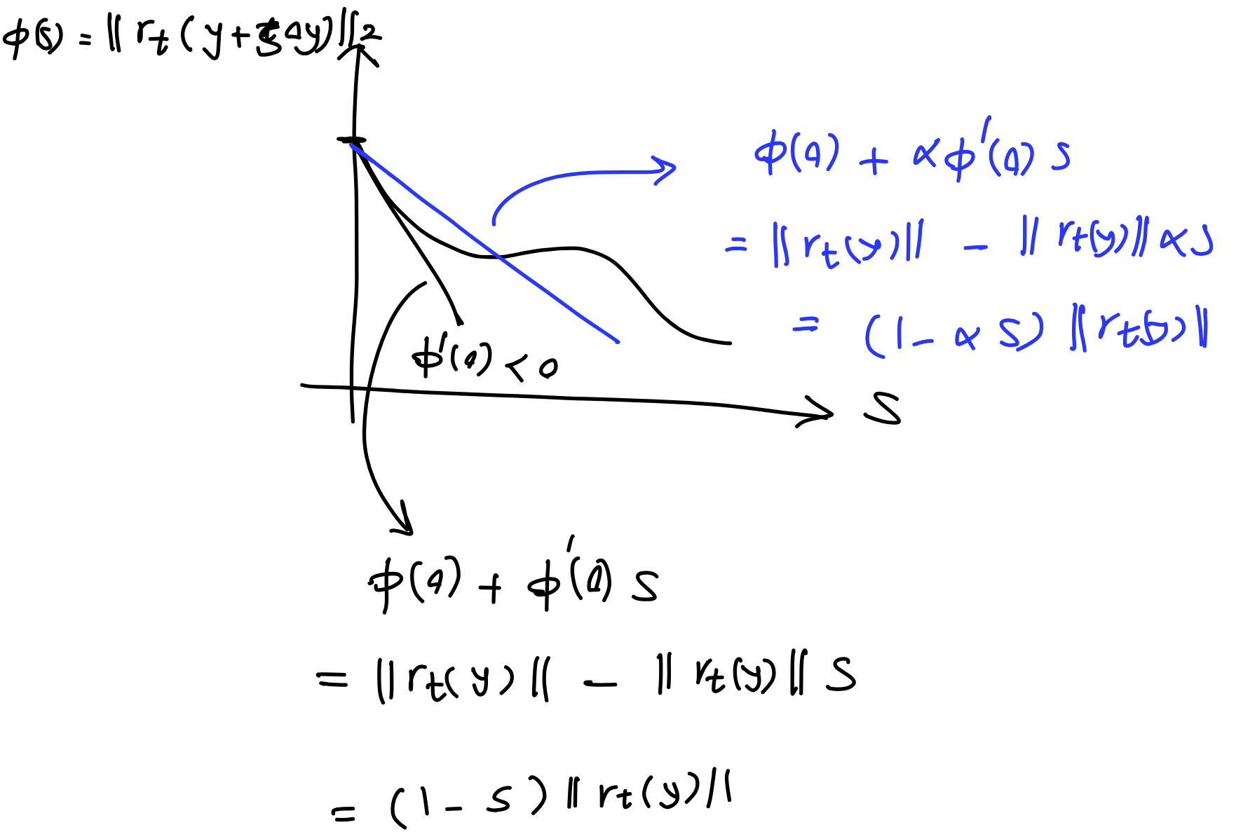
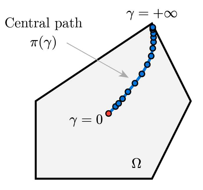
Tangent to central path
We consider the central path $x^\star(t) = \arg\min_{x}\; t f_0(x) + \phi(x),$ which, by optimality, satisfies the centrality (stationarity) equation $t \nabla f_0\bigl(x^\star(t)\bigr) + \nabla \phi\bigl(x^\star(t)\bigr) = 0.$
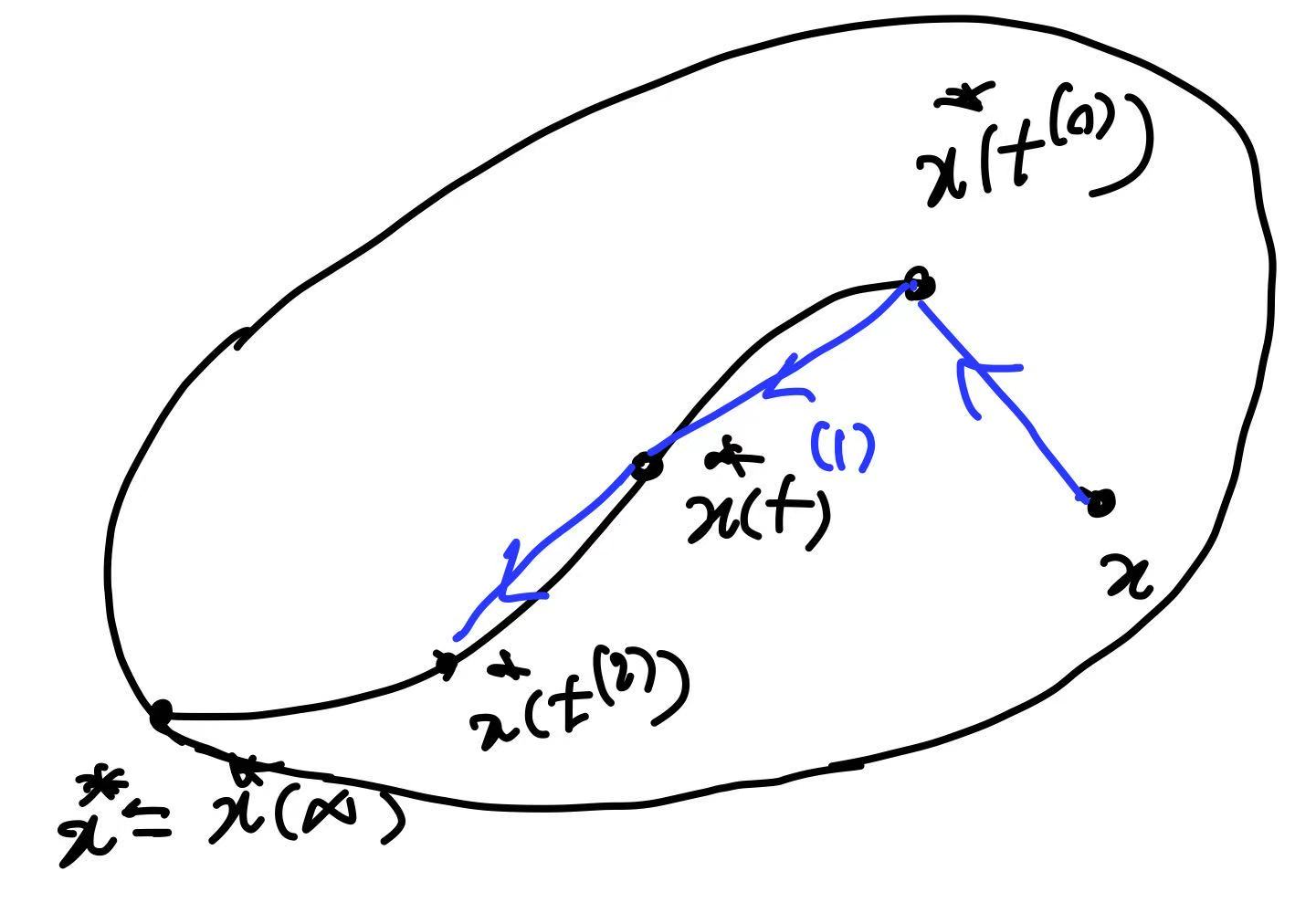
Viewing this equation as an implicit definition of $x^\star(t)$ as a function of $t$, implicit differentiation with respect to $t$ yields the tangent direction along the central path:
\[\frac{d x^\star(t)}{d t} = -\Bigl(t \nabla^2 f_0\bigl(x^\star(t)\bigr) + \nabla^2 \phi\bigl(x^\star(t)\bigr)\Bigr)^{-1} \nabla f_0\bigl(x^\star(t)\bigr).\]Consequently, the first-order predictor obtained by increasing $t$ from $t$ to $\mu t$ is
\[\hat{x} = x^\star(t) + \frac{d x^\star(t)}{d t}(\mu t - t)\]which simply approximates $x^\star(\mu t)$ by moving along the tangent of the central path.
Since we use surrogate duality gap to evaluate duality gap, $\hat{\eta} = s^\top \lambda$ and $\bar{\eta} = \hat{\eta}/m$, a more natural way is to treat central path and decision variable as implicit functions of $\bar{\eta}$ and use tangent line as predictor
\[\mathcal{X}(\bar{\eta}^+) \approx \mathcal{X}(\bar{\eta}) + \frac{d \mathcal{X}^\star}{d \bar{\eta}} \bigl(\bar{\eta}^+ - \bar{\eta}\bigr).\]On the central path, $s_i \lambda_i = 1/t$, therefore $\bar{\eta} = 1/t$. Hence, $t^+ = \mu t \Longleftrightarrow \bar{\eta}^+ = \bar{\eta}/\mu$. That is the outer update rather driving down the gap scale $\bar{\eta}$. We write the central path as an implicit equation parameterized by $\bar{\eta}$:
\[r(x,s,\lambda,\nu;\bar{\eta}) = \begin{bmatrix} r_{\mathrm{dual}} \\ r_{\mathrm{cent}}(\bar{\eta}) \\ r_{\mathrm{pri,ineq}} \\ r_{\mathrm{pri,eq}} \end{bmatrix} = \begin{bmatrix} Qx + q + G^\top \lambda + A^\top \nu \\ \mathrm{diag}(s)\lambda - \bar{\eta}\mathbf{1} \\ Gx + s - h \\ Ax - b \end{bmatrix} = 0.\]Differentiate $r(\mathcal{X}^\star;\bar{\eta}) = 0$ with respect to $\bar{\eta}$ using implicit function theorem:
\[D_{\mathcal{X}} r(\mathcal{X};\bar{\eta})\,\frac{d\mathcal{X}^\star(\bar{\eta})}{d\bar{\eta}} + \frac{\partial r}{\partial \bar{\eta}} = 0.\]Note that only $r_{\mathrm{cent}}$ depends on $\bar{\eta}$, so $\partial r/\partial \bar{\eta}=[0,-\mathbf{1},0,0]^{\top}$. $D_{\mathcal{X}} r$ is the KKT Jacobian block above, and tangent vector satisfy :
\[D_{\mathcal{X}} r= \begin{bmatrix} Q & 0 & G^\top & A^\top\\ 0 & \operatorname{diag}(\lambda) & \operatorname{diag}(s) & 0\\ G & I & 0 & 0\\ A & 0 & 0 & 0 \end{bmatrix}, \quad D_{\mathcal{X}} r \cdot\frac{d\mathcal{X}^\star(\bar{\eta})}{d\bar{\eta}}=\begin{bmatrix} 0\\ \mathbf{1}\\ 0\\ 0 \end{bmatrix}\]From the Tangent to the Affine-Scaling Predictor: Mehrotra’s First Step
Now let’s first construct an aggressive predictor by setting an extreme target: take the next step directly to $\bar{\eta}^{+}=0$ , drive the average complementarity directly to zero, reduce the complementarity without any explicit centering.
If the current point is near the central path:$r_{\mathrm{dual}} \approx r_{\mathrm{pri}} \approx 0,\quad \mathrm{diag}(s)\lambda \approx \bar{\eta}\mathbf{1}.$
Then the tangent step corresponding to pushing $\bar{\eta}$ from its current value to $0$ is simply
\[\Delta\bar{\eta} = -\bar{\eta}.\]Plugging into the tangent equation gives (on the central path, $\bar{\eta}\mathbf{1}=\mathrm{diag}(s)\lambda$):
\[\begin{bmatrix} Q & 0 & G^\top & A^\top\\ 0 & \operatorname{diag}(\lambda) & \operatorname{diag}(s) & 0\\ G & I & 0 & 0\\ A & 0 & 0 & 0 \end{bmatrix}\,\Delta\mathcal{X} = \begin{bmatrix} 0\\ 1\\ 0\\ 0 \end{bmatrix}\Delta\bar{\eta} = \begin{bmatrix} 0\\ -\bar{\eta}\mathbf{1}\\ 0\\ 0 \end{bmatrix} = \begin{bmatrix} 0\\ -\mathrm{diag}(s)\lambda\\ 0\\ 0 \end{bmatrix} = \begin{bmatrix} 0\\ -\,s\circ\lambda\\ 0\\ 0 \end{bmatrix}.\]This explains why Mehrotra Step uses $-\mathrm{diag}(s)\lambda$ in Mehrotra’s first (Newton-like) step: it is the direction that predicts along the central-path tangent pushing $\bar{\eta}$ toward $0$ (and it matches exactly on the central path).
Away from the central path, we must simultaneously reduce the primal and dual residuals $r_{\mathrm{dual}}, r_{\mathrm{pri}}$ simultaneously, so the affine predictor actually solves the linear system:
\[\begin{bmatrix} Q & 0 & G^\top & A^\top\\ 0 & \operatorname{diag}(\lambda) & \operatorname{diag}(s) & 0\\ G & I & 0 & 0\\ A & 0 & 0 & 0 \end{bmatrix} \begin{bmatrix} \Delta x^{\mathrm{aff}}\\ \Delta s^{\mathrm{aff}}\\ \Delta \lambda^{\mathrm{aff}}\\ \Delta \nu^{\mathrm{aff}} \end{bmatrix} = - \begin{bmatrix} r_{\mathrm{dual}}\\ \mathrm{diag}(s)\lambda\\ r_{\mathrm{pri,ineq}}\\ r_{\mathrm{pri,eq}} \end{bmatrix}.\]Line search for affine-scaling predictor is exactly same as the one for original newton step:
\[\alpha^{\mathrm{aff}} \leftarrow 0.99\,\alpha_{\max}^{\mathrm{aff}}, \quad \alpha_{\max}^{\mathrm{aff}} = \min\Bigl( 1,\ \min_{i:\Delta s^{\mathrm{aff}}_i<0}\Bigl(-\frac{s_i}{\Delta s^{\mathrm{aff}}_i}\Bigr),\ \min_{i:\Delta\lambda^{\mathrm{aff}}_i<0}\Bigl(-\frac{\lambda_i}{\Delta\lambda^{\mathrm{aff}}_i}\Bigr) \Bigr).\]So the predicted surrogate duality gap at the affine step is:
\[\hat{\eta}^{\mathrm{aff}} := \bigl(s+\alpha^{\mathrm{aff}}\Delta s^{\mathrm{aff}}\bigr)^\top \bigl(\lambda+\alpha^{\mathrm{aff}}\Delta \lambda^{\mathrm{aff}}\bigr), \quad \bar{\eta}^{\mathrm{aff}} := \frac{\hat{\eta}^{\mathrm{aff}}}{m}.\]Second Step: Centering-plus-corrector Directions
Mehrotra’s second step uses the affine predictor to choose an adaptive centering strength:
\[\sigma = \left(\frac{\hat{\eta}^{\mathrm{aff}}}{\hat{\eta}}\right)^3 = \left( \frac{\bigl(s+\alpha^{\mathrm{aff}}\Delta s^{\mathrm{aff}}\bigr)^\top \bigl(\lambda+\alpha^{\mathrm{aff}}\Delta \lambda^{\mathrm{aff}}\bigr)} {s^\top \lambda} \right)^{3} ,\]to adaptively decide how much “centering” to enforce in the next step (Or $\sigma$ can be set by heuristic, smaller $\sigma$ is more aggressive; larger $\sigma$ is more conservative, pulling harder back toward the center).This changes a key point of original PD-IPM: we originally hand-fixed the outer growth factor $\mu$; Mehrotra uses the affine predictor to automatically estimate how small it can drive $\bar{\eta}$, and then backs out an appropriate centering strength $\sigma$.
Therefore the new centering target we want (componentwise) is
\[s_i^{+}\lambda_i^{+} \approx \sigma\bar{\eta},\quad i=1,\ldots,m, \quad (s+\Delta s)\circ(\lambda+\Delta\lambda)\approx \sigma\bar{\eta}\mathbf{1}\]Expanding elementwise gives
\[s\circ\lambda +\mathrm{diag}(s)\Delta\lambda +\mathrm{diag}(\lambda)\Delta s +(\Delta s\circ\Delta\lambda) =\sigma\bar{\eta}\mathbf{1}.\]A standard Newton linearization drops the second-order term $\Delta s\circ\Delta\lambda$: $\mathrm{diag}(s)\Delta\lambda +\mathrm{diag}(\lambda)\Delta s =\sigma\bar{\eta}\mathbf{1}-s\circ\lambda.$ The affine predictor corresponds exactly to this linearized equation with $\sigma=0$: $ \mathrm{diag}(s)\Delta\lambda^{\mathrm{aff}} +\mathrm{diag}(\lambda)\Delta s^{\mathrm{aff}} =-\,s\circ\lambda.$
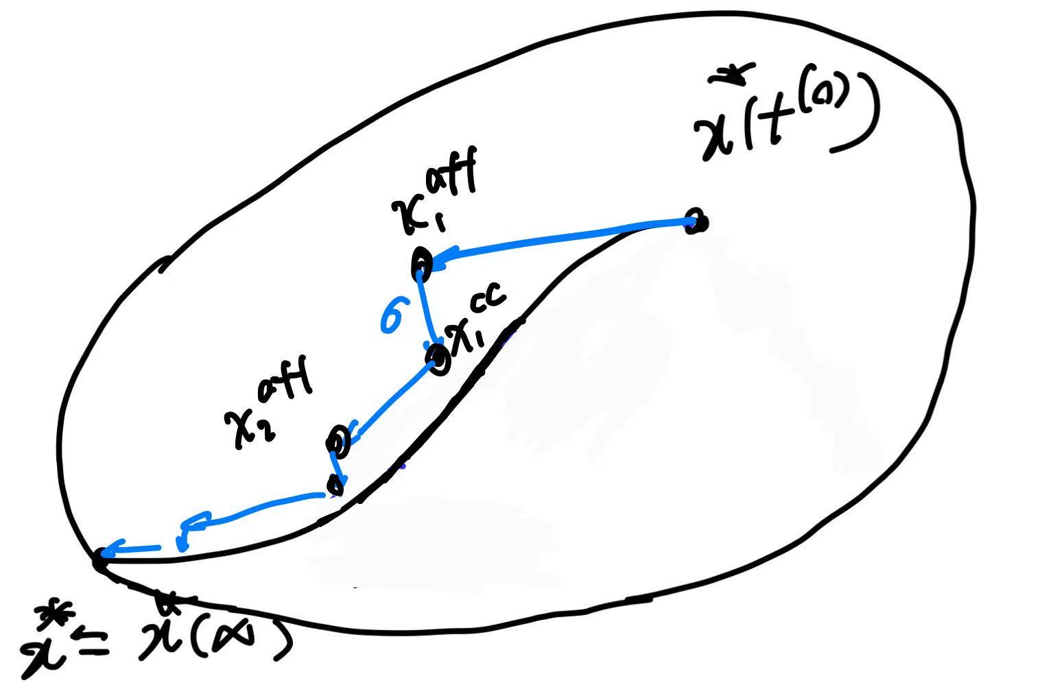
Although the affine predictor makes the linearized complementarity residual small, the true complementarity at the affine step contains the quadratic term $\Delta s^{\mathrm{aff}}\circ\Delta\lambda^{\mathrm{aff}}$, which can be large and typically pushes the iterates toward the boundary. The corrector modifies the complementarity equation by (i) shifting the target from $0$ to $\sigma\bar{\eta}\mathbf{1}$ (centering) $ \mathrm{diag}(s)\Delta\lambda^{\mathrm{cc}} +\mathrm{diag}(\lambda)\Delta s^{\mathrm{cc}} =\sigma\bar{\eta}\mathbf{1}. $
and (ii) subtracting the estimated quadratic error (corrector) $\Delta s\circ\Delta\lambda\approx\Delta s^{\mathrm{aff}}\circ\Delta\lambda^{\mathrm{aff}}.$
Therefore, plug into $s\circ\lambda+\mathrm{diag}(s)\Delta\lambda+\mathrm{diag}(\lambda)\Delta s+(\Delta s\circ\Delta\lambda)=\sigma\bar{\eta}\mathbf{1},\; \mathrm{diag}(s)\Delta\lambda^{\mathrm{aff}} +\mathrm{diag}(\lambda)\Delta s^{\mathrm{aff}} =-\,s\circ\lambda,$ the centering block in the corrector becomes
\[\mathrm{diag}(s)\Delta\lambda^{\mathrm{cc}} +\mathrm{diag}(\lambda)\Delta s^{\mathrm{cc}} = \sigma\bar{\eta}\mathbf{1} - \bigl(\Delta s^{\mathrm{aff}}\circ\Delta\lambda^{\mathrm{aff}}\bigr).\]So the centering-plus-corrector directions solves linear system
\[\begin{bmatrix} Q & 0 & G^\top & A^\top\\ 0 & \operatorname{diag}(\lambda) & \operatorname{diag}(s) & 0\\ G & I & 0 & 0\\ A & 0 & 0 & 0 \end{bmatrix} \begin{bmatrix} \Delta x^{\mathrm{cc}}\\ \Delta s^{\mathrm{cc}}\\ \Delta\lambda^{\mathrm{cc}}\\ \Delta\nu^{\mathrm{cc}} \end{bmatrix} = \begin{bmatrix} 0\\ \sigma\bar{\eta}\mathbf{1} - \mathrm{diag}(\Delta s^{\mathrm{aff}})\Delta\lambda^{\mathrm{aff}}\\ 0\\ 0 \end{bmatrix}.\]The final combined search direction is then $\Delta\mathcal X=\Delta\mathcal X^{\mathrm{aff}}+\Delta\mathcal X^{\mathrm{cc}},$ explcitly conbime two direction vectors:
\[\begin{bmatrix} \Delta x \\ \Delta s \\ \Delta \lambda \\ \Delta \nu \end{bmatrix} = \begin{bmatrix} \Delta x^{\mathrm{aff}} \\ \Delta s^{\mathrm{aff}} \\ \Delta \lambda^{\mathrm{aff}} \\ \Delta \nu^{\mathrm{aff}} \end{bmatrix} + \begin{bmatrix} \Delta x^{\mathrm{cc}} \\ \Delta s^{\mathrm{cc}} \\ \Delta \lambda^{\mathrm{cc}} \\ \Delta \nu^{\mathrm{cc}} \end{bmatrix}.\]Given $\Delta\mathcal X$, line search is same as previous enforcing interior feasibility, explicitly
\[\alpha = \min\left\{ 1,\; 0.99 \sup\left\{ \alpha \ge 0 \ \middle|\ s + \alpha\,\Delta s \ge 0,\ \lambda + \alpha\,\Delta \lambda \ge 0 \right\} \right\}.\]Now update the primal and dual variables $\mathcal X^{+}=\mathcal X+\alpha\,\Delta\mathcal X$.
Initialization
Following [5] Section 5 Path-following algorithm for cone QPs, primal and dual starting points are selected as follows:
Here solve the analytical solution for the primal problem:
\[\begin{aligned} \min_{x,s}\quad & \frac{1}{2}x^\top Qx + q^\top x + \frac{1}{2}\|s\|_2^2\\ \text{s.t.}\quad & Gx + s = h,\\ & Ax = b, \end{aligned}\]which can be written as the block system
\[\begin{bmatrix} Q & G^\top & A^\top\\ G & -I & 0\\ A & 0 & 0 \end{bmatrix} \begin{bmatrix} x\\ \lambda\\ \nu \end{bmatrix} = \begin{bmatrix} -q\\ h\\ b \end{bmatrix}.\]The dual problem is
\[\begin{aligned} \max_{w,\lambda,\nu}\quad & -\frac{1}{2}w^\top Qw - h^\top \lambda - b^\top \nu - \frac{1}{2}\|\lambda\|_2^2\\ \text{s.t.}\quad & Qw + q + G^\top \lambda + A^\top \nu = 0. \end{aligned}\]This initialization solves a different, regularized primal–dual pair and serves as a generic, numerically stable way to generate a strictly interior starting point. The added norm terms tend to keep the slack magnitude moderate—so the implied inequality violation as measured by $\lVert s \rVert_2^2,\lVert \lambda \rVert_2^2$ in primal-dual problem is typically not extreme—but the construction is not intended to provide a starting point that is necessarily close to the optimal solution.
Now shift the linear system solution to a strictly interior starting point. After solving the regularized equality-constrained system to obtain provisional $(x^{(0)},\nu^{(0)})$, we form the inequality residual
\[r := Gx^{(0)} - h\]Define the minimum shifts that make the slack and multiplier nonnegative componentwise:
\[\alpha_p := \inf\{\alpha\in\mathbb{R}\mid -r + \alpha \mathbf{1} \ge \mathbf{0}\},\qquad \alpha_d := \inf\{\alpha\in\mathbb{R}\mid \;\;r + \alpha \mathbf{1} \ge \mathbf{0}\}.\]then set
\[s^{(0)} := \begin{cases} -r, & \alpha_p < 0,\\ -r + (1+\alpha_p)\mathbf{1}, & \text{otherwise}, \end{cases} \qquad \lambda^{(0)} := \begin{cases} r, & \alpha_d < 0,\\ r + (1+\alpha_d)\mathbf{1}, & \text{otherwise}. \end{cases}\]This simple shift guarantees a strictly interior initialization $s^{(0)}>\mathbf{0}$ and $\lambda^{(0)}>\mathbf{0}$, yielding the starting point $\mathcal{X}^{(0)} := \bigl[x^{(0)},\, s^{(0)},\, \lambda^{(0)},\, \nu^{(0)}\bigr]^\top$.
At each iteration,
1) check termination based on primal/dual residual norms and the surrogate duality gap;
2) compute an affine-scaling predictor search direction.
3) compute a centering-plus-corrector direction;
4) backtracking line search in residuals;
5) update the primal and dual variables and repeat.
Result for simple QP


Future work
Nearly all of the computational effort is in the solution of the linear systems in steps 2 and 3 which detailed introduced above. Both linear systems have same LHS with same structured KKT matrix. Numerical factorization can be futher explored.
References
[1]. Boyd, S. & Vandenberghe, L. Convex Optimization. Cambridge University Press, 2004.
[2]. Mattingley, J. & Boyd, S. CVXGEN: a code generator for embedded convex optimization, Optimization and Engineering, vol. 13, no. 1, pp. 1-27, 2012.
[3]. Pandala, A. G., Ding, Y., & Park, H.-W. qpSWIFT: A Real-Time Sparse Quadratic Program Solver for Robotic Applications, IEEE Robotics and Automation Letters, vol. 4, no. 4, pp. 3355–3362, Oct. 2019. doi:10.1109/LRA.2019.2926664
[4]. Mehrotra, S. On the Implementation of a Primal-Dual Interior Point Method, SIAM Journal on Optimization, vol. 2, no. 4, pp. 575–601, 1992. doi:10.1137/0802028
[5]. Vandenberghe, L. The CVXOPT linear and quadratic cone program solvers. Technical report / notes, March 20, 2010. https://www.seas.ucla.edu/~vandenbe/publications/coneprog.pdf