Trajectory Optimization with Orientations
Quaternion optimal control with acados, kRRT on manifold, combinatorial optimization
Astrobee attitude-slew MPC
This project gave me a much clearer intuition for unit quaternions and Lie-group formulation as parameterizations of attitude. It is important that the cost be invariant to the sign of the quaternion because of topological identification property $q \sim -q$ and reflect the true relative rotation angle. In the Astrobee attitude-slew MPC below, cost was firstly built from the scalar product $q^\top q_g$,
\[e_q = 1 - (q^\top q_g)^2.\]After increasing the terminal weight on this attitude error term, the MPC drives Astrobee to the desired attitude with small residual angular rates as in the figure.
\[\begin{aligned} \min_{\{q_k, \omega_k, M_k\}_{k=0}^{N-1}} \quad & \sum_{k=0}^{N-1} \Big( Q_q\,\big[1 - (q_k^\top q_g)^2\big] + \omega_k^\top Q_\omega\, \omega_k + M_k^\top R\, M_k \Big) \\ &\quad + Q_q^N\,\big[1 - (q_N^\top q_g)^2\big] + \omega_N^\top Q_\omega^N\, \omega_N \\[0.5em] \text{s.t.} \quad & q_{k+1} = \frac{q_k + \tfrac{1}{2}\,\Omega(\omega_k)\, q_k\, \Delta t} {\big\|q_k + \tfrac{1}{2}\,\Omega(\omega_k)\, q_k\, \Delta t\big\|}, \qquad k = 0,\dots, N-1, \\[0.3em] & \omega_{k+1} = \omega_k + \Delta t\, J^{-1}\!\big( M_k - \omega_k \times (J \omega_k) \big), \qquad k = 0,\dots, N-1, \\[0.3em] & \| \omega_k \|_\infty \le \omega_{\max}, \quad \| M_k \|_\infty \le M_{\max}, \qquad k = 0,\dots, N-1, \\[0.3em] & q_0 = q_{\mathrm{init}}, \quad \omega_0 = \omega_{\mathrm{init}}, \quad q_k \in S^3, \ \omega_k, M_k \in \mathbb{R}^3. \end{aligned}\], where \(\Omega(\omega) = \begin{bmatrix} 0 & -\omega^\top \\ \omega & -[\omega]_\times \end{bmatrix}.\)
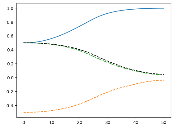
The MPC problem above is implemented in acados OCP class using a multiple-shooting SQP based on HPIPM with a small L-M regularization. With an initial $q_0 = [0.5,\,-0.5,\,0.5,\,0.5]$ and goal $q_g = [1,0,0,0]$, the plot shows the resulting quaternion attitude trajectories.
Lie-group-theoretic nonholonomic RRT for flexible needle
Replacing the quaternion orientation residual with the intrinsic geodesic cost $|(\log(R_{\text{goal}}^\top R))^\vee|^2$ noticeably improves optimization in practice, even without a large terminal penalty. Motivated by this, the next project explores Lie-group methods on $SE(2)$ for geometry-aware planning.
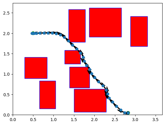
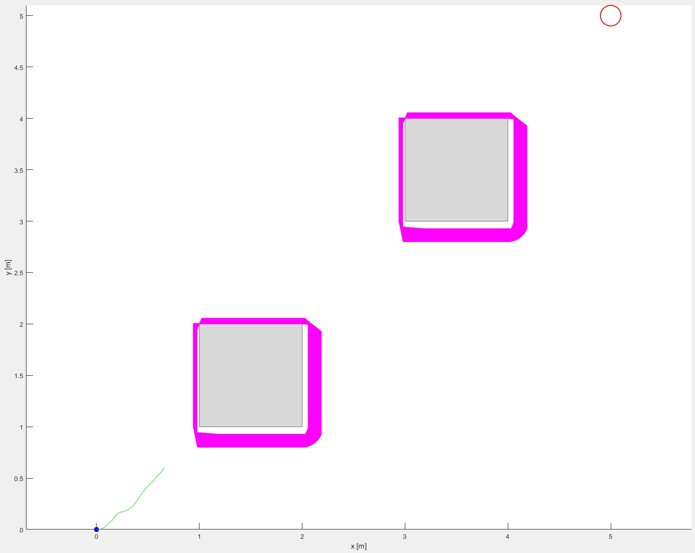
We implement a Lie-group nonholonomic RRT on $SE(2)$ for a flexible-needle unicycle model with state $q=(x,y,\theta)^\top\in\mathbb R^2\times S^1$ and control $u=(u_\phi,u_\omega)^\top$, where $u_\phi$ is wheel (needle) angular speed and $u_\omega$ is yaw rate. The kinematics are $\dot x=r\,u_\phi\cos\theta,\ \dot y=r\,u_\phi\sin\theta,\ \dot\theta=u_\omega$, i.e. $\dot q=B(q)u$.
Let $g\in SE(2)$ be the pose and define the body twist $V^{\mathrm b}=\xi^{\mathrm b}=(g^{-1}\dot g)^\vee=(v_x^{\mathrm b},v_y^{\mathrm b},\omega)^\top =J^b(q)\dot q=J^b(q)B(q)u$ with body Jacobian $J^b(q)$, yielding $\xi=(g^{-1}\dot g)^\vee=(r\,u_\phi,0,u_\omega)^\top$ and the corresponding Lie-theoretic control–affine model $\dot g=g\hat\xi$. For piecewise-constant $u$, the exact update is $g(t+\Delta t)=g(t)\exp(\hat\xi\,\Delta t)$.
In the RRT, each extension evaluates a finite control set $u\in\mathcal U_d$ and propagates the nearest node via the exact Lie-group step $g_{k+1}=g_k\exp(\hat\xi(u)\Delta t)$, rather than Euler/RK4.
Combinatorial optimization