Continuous-time Successive Convexification

← Back

The standard formulation of nonlinear optimal control infinite-dimensional problems, minimizing a cost functional subject to continuous-time dynamics $\dot{x}(t) = f(x(t), u(t))$ and inequality constraints $g(x(t), u(t)) \le 0$ over $t \in [0, t_f]$, typically relies heavily on time-discretization. To achieve computational tractability, traditional direct methods and Sequential Convex Programming (SCP) algorithms relax these continuous path constraints, enforcing them exclusively at a finite set of discrete nodes, $t_k$.

While this node-only enforcement yields tractable subproblems solvable by direct methods, it inherently misses inter-sample constraint violations, which can render mathematically optimal trajectories physically unsafe in critical scenarios like obstacle avoidance. Trivially increasing the grid density to catch these blind spots only destroys real-time performance. To break this resolution-versus-safety trade-off, this project explores the Continuous-Time Successive Convexification (CT-SCvx) framework in [1]. By introducing an augmented state to continuously integrate and accumulate constraint violations, CT-SCvx transforms point-wise constraints into an exact continuous-time penalty. This paradigm shift guarantees rigorous constraint satisfaction across the entire continuous-time domain, \( [0, t_f] \), entirely independent of the temporal grid resolution.

Problem Formulation

To address continuous-time constraint satisfaction, we consider nonlinear optimal control problems (OCPs) in the Mayer-Bolza form. Let $x(t) \in \mathbb{R}^{n_x}$ and $u(t) \in \mathbb{R}^{n_u}$ denote the state trajectory and control input, respectively. The OCP is formulated as:

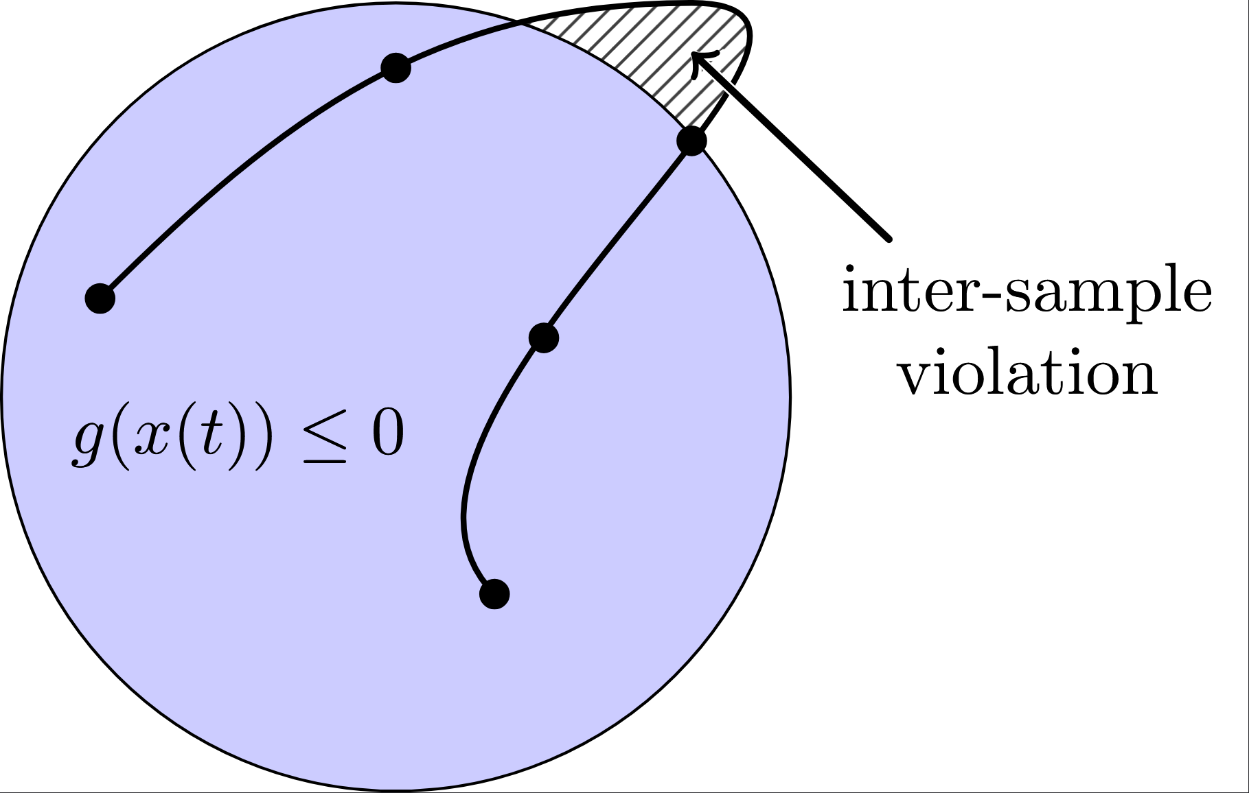
where $f$ defines the system dynamics, $g$ represents nonlinear inequality constraints, and $\mathcal{U} \subset \mathbb{R}^{n_u}$ is a simple convex set of admissible controls. Standard direct methods typically enforce path constraints only at discrete time nodes, which invariably leads to inter-sample violations. To ensure feasibility across the entire continuous-time horizon, we employ an exact penalization paradigm by introducing a smooth monotonic increase exterior penalty function $ \Lambda: \mathbb{R}^{n_x} \times \mathbb{R}^{n_u} \to \mathbb{R}_+ $:

By augmenting the state vector with the cumulative running cost and the constraint violation metric, $\bar{x} = (x, y, \mathcal{L}) \in \mathbb{R}^{n_x+2}$, the augmented dynamics are given by:

Under this paradigm, enforcing continuous-time path constraints is equivalent to ensuring the terminal state condition $y(t_f) = \int_{0}^{t_f} \Lambda(x(t), u(t)) \, dt = 0$. This transformation enables the use of convergence-guaranteed algorithms, such as the prox-linear method, to solve the reformulated problem efficiently.

Multiple-Shooting Discretization & First-Order Sensitivities via Variational ODEs

We now parameterize continuous-time infinitely-dimensional optimization as a multiple-shooting finitely-dimensional trajectory optimization problem. We define a temporal grid $0 = t_1 < t_2 < \dots < t_N = t_f$ and parameterize the control trajectory $u(t)$ as a piecewise constant signal—a Zero-Order Hold (ZOH) representation, where $u(t) = \eta_k$ for $t \in [t_k, t_{k+1})$ and $\eta_k \in \mathbb{R}^{n_u}$ denotes the decision variables for control. Let $\xi_k \in \mathbb{R}^{n_{\bar{x}}}$ represent the augmented state at node $t_k$. We define the flow map $F_k: \mathbb{R}^{n_{\bar{x}}} \times \mathbb{R}^{n_u} \to \mathbb{R}^{n_{\bar{x}}}$ as the integral solution of the augmented dynamics:

where $\bar{x}(\tau)$ is the solution to the initial value problem (IVP) $\dot{\bar{x}} = \bar{f}(\bar{x}, \eta_k)$ with $\bar{x}(t_k) = \xi_k$. The OCP is thus transcribed into a finite-dimensional program constrained by the discrete transitions $\xi_{k+1} = F_k(\xi_k, \eta_k)$. Assuming an ideal ODE solver, this multiple-shooting formulation is numerically exact , as it transcribes the continuous vector field into its integral representation without the local truncation errors or topological artifacts typical of fixed-step discretizations.

A core prerequisite for sequential convexification is linearizing the highly nonlinear flow map $F_k$ about a nominal trajectory $(\tilde\xi_k, \tilde\eta_k)$ to formulate convex subproblemsconstraints, especially since there is no closed-form formula for the function $F_k$. Direct finite-differencing of the numerical integration is fundamentally flawed due to ill-conditioning and computational inefficiency. CT-SCvx extracts the analytical first-order gradients by using the theory of variational ordinary differential equations. Our goal is to compute the state transition matrix $A_k \in \mathbb{R}^{n_{\bar{x}} \times n_{\bar{x}}}$ and the input sensitivity matrix $B_k \in \mathbb{R}^{n_{\bar{x}} \times n_u}$, defined respectively as the Jacobians of the flow map:

Let $\Phi_{\bar{x}}(t)$ and $\Phi_{u}(t)$ be the continuous sensitivity matrices. According to the variational principle, their temporal evolution is governed by the Jacobians of the augmented continuous vector field $\bar{f}$, evaluated along the nominal trajectory. These matrices satisfy the following coupled IVP over $t \in [t_k, t_{k+1}]$:

By stacking the augmented state, $\Phi_{\bar{x}}(t)$, and $\Phi_u(t)$ into a single enlarged ODE system, and jointly integrating them from $t_k$ to $t_{k+1}$ using a high-fidelity ODE solver, the exact discrete Jacobians naturally precipitate at the terminal boundary:

This mechanism transforms the intractable infinite-dimensional mapping into an exact, piecewise-affine relation $\xi_{k+1} \approx A_k \xi_k + B_k \eta_k + c_k$. It forms the backbone of the computational efficiency of CT-SCvx, providing mathematically immaculate first-order gradient information to drive the downstream Prox-Linear optimization without compromising the rigorous continuous-time physics.

In this multiple-shooting transcription, let $y_k$ denote the $y$-component of the discrete augmented state $\xi_k$. The $y$-state enforces the accumulated constraint violation via the discrete transition and a natural way to encode continuous-time feasibility is to additionally impose that no violation accumulates over any interval:

However, imposing both constraints simultaneously creates a structural redundancy at feasibility, which inevitably violates the Linear Independence Constraint Qualification (LICQ). Since if both constraints hold strictly, then

Because $\Lambda \ge 0$ by definition, this implies $\Lambda(x(t), \eta_k) = 0$ almost everywhere on $[t_k, t_{k+1}]$. For the squared-hinge penalty $\Lambda = \frac{1}{2}|\max{g(x), 0_{n_g}}|_2^2$, this further dictates that the partial derivatives $\frac{\partial \Lambda}{\partial x}$ and $\frac{\partial \Lambda}{\partial u}$ are exactly zero almost everywhere along that interval.

Consequently, the row in the state transition Jacobian ($A_k$) corresponding to the $y$-dynamics loses all sensitivity to $x$ and $u$. It collapses to simply $+1$ with respect to $y_{k+1}$ and $-1$ with respect to $y_k$. This results in a gradient vector that is mathematically identical to the gradient of the strict path constraint $y_{k+1} - y_k = 0$. When two active constraints share the exact same gradient, LICQ inherently fails, paralyzing downstream gradient-based solvers. To eliminate this built-in degeneracy, the strict per-interval equality is relaxed to a small bounded inequality:

If it is inactive ($y_{k+1} - y_k < \epsilon$), the constraint drops out of the active set altogether, and its gradient does not threaten linear independence. If it is active ($y_{k+1} - y_k = \epsilon$), the $y$-dynamics force the integral to evaluate to exactly $\epsilon > 0$. This strict positivity implies that $\Lambda > 0$ on some sub-interval, which in turn “awakens” the non-zero gradients $\frac{\partial \Lambda}{\partial x}$ and $\frac{\partial \Lambda}{\partial u}$. The $y$-dynamics Jacobian now contains additional $(x, u)$-dependence, ensuring it is no longer identical to the relaxed constraint’s Jacobian. By ensuring LICQ is no longer trivially violated, this $\epsilon$-relaxation enables the exact-penalty and prox-linear machinery to function in a numerically well-posed and theoretically sound environment.

Reformulated relaxed optimal control problem is as follows

$\ell_1$ Exact Penalization and the Prox-Linear Method

Following the multiple-shooting discretization, the continuous-time optimal control problem is transcribed into a non-convex, finite-dimensional Nonlinear Programming (NLP) problem. The prox-linear method can solve this efficiently, an iterative algorithm that relies on exact penalization to transform the intractable NLP into a sequence of strongly convex subproblems. It relax the dynamics constraint and penalize the violation using an $\ell_1$-norm exact penalty. Conceptually, augment the objective function with the sum of the absolute dynamics errors:

The exact penalty theorem guarantees that if the penalty parameter $\gamma > 0$ exceeds a certain finite threshold, the local minimizers of this relaxed, unconstrained problem coincide precisely with those of the strictly constrained NLP. The solver is allowed to temporarily violate the dynamics to find a path, progressively driving the errors to zero as the trajectory converges.

However, the $\ell_1$-norm is non-smooth (non-differentiable at zero), which prevents the direct use of high-speed interior-point solvers like MOSEK or SCS. To resolve this, we smoothly reformulate the $\ell_1$-norm by splitting the error into non-negative slack variables: $q_k > 0 \in \mathbb{R}^{n_{\bar{x}}}$ for positive deviations and $r_k > 0 \in \mathbb{R}^{n_{\bar{x}}}$ for negative deviations. The dynamics error is exactly captured by $\xi_{k+1} - (A_k \xi_k + B_k \eta_k + c_k) = q_k - r_k$, and the $\ell_1$-norm translates linearly to $\mathbf{1}^\top (q_k + r_k)$.

Because the affine approximation of the flow map is only valid within a local neighborhood of the nominal trajectory $(\tilde{\xi}, \tilde{\eta})$, taking excessively large optimization steps can invalidate the linearization and cause divergence. We counteract this by augmenting the cost function with a proximal regularization term, scaled by $\rho > 0$, which effectively establishes a trust-region.

Combining the original Mayer cost, the smoothly reformulated exact penalty, and the proximal regularization, the resulting strictly convex subproblem solved at each sequential iteration is formulated as:

This prox-linear formulation structurally guarantees recursive feasibility. By reducing the intractable NLP into a sequence of QPs, the algorithm naturally drives the slack variables $q_k, r_k$ to zero as the proximal steps shrink, ultimately yielding a dynamically feasible and mathematically rigorous optimal trajectory.

While the prox-linear method with exact penalization provides strong theoretical guarantees, its static penalty parameters are notoriously difficult to tune for complex nonlinear dynamics like the cart-pole system. For practical engineering implementation, here transition to a primal-dual Augmented Lagrangian Method (ALM). By employing dynamic Lagrange multipliers alongside a smooth quadratic penalty to strictly penalize constraint violations, ALM achieves exact feasibility without requiring manual tuning of the penalty weights.

where $Z := \big[\xi_1^\top,\ldots,\xi_N^\top,\eta_1^\top,\ldots,\eta_{N-1}^\top\big]^\top$ is the stacked decision vector; $c(Z)$ stacks all equality residuals; $g(Z)$ stacks all inequality residuals. To solve the resulting unconstrained subproblems, we deploy the L-BFGS algorithm. Its inherent line-search mechanism naturally regulates the update step size, implicitly replacing the manually tuned proximal trust-region parameter and yielding a robust, tuning-free architecture.

To validate the continuous-time safety of the framework, we evaluate it on two optimal control tasks. The first is a 2D double integrator obstacle avoidance problem. As demonstrated in the spatial trajectory and the corresponding constraint evaluation , the standard node-only baseline satisfies the constraint solely at discrete sampling nodes, mathematically permitting inter-sample collisions with the obstacle. In contrast, CT-SCvx rigorously ensures the entire continuous trajectory remains strictly outside the exclusionary zone.

The second example considers a highly nonlinear cart–pole swing-up problem with strict spatial constraints. For comparison, a node-only transcription, where both the dynamics and continuous inequality constraints are discretized via RK4 and solved using direct method, exhibits constraint violations between discrete time nodes. In contrast, CT-SCvx rigorously enforces continuous-time feasibility, keeping the entire trajectory within the prescribed bounds and completing the swing-up without any inter-sample constraint violation. For comparison, both methods export their ZOH control inputs and are simulated using a high-accuracy ODE integrator; under this continuous-time evaluation, CT-SCvx demonstrates significantly improved continuous-time dynamics and constraint satisfaction.

Direct method and shooting method

For comparison/reference to successive convexification, this section briefly introduces the direct transcription method and the shooting method. The shooting method (in following) does not achieve particularly high performance on the cart–pole system swing-up task. The most apparent issue is the final few time steps, the control inputs fail to precisely drive both the cart and the pole velocities to zero. Fundamentally, shooting method requires computing high powers of the system matrix $A^{n}$, causing the early control input $u_{[0]}$ to exert a much stronger influence on the overall trajectory and cost than the later control input $u_{[N−1]}$. Additionally, direct transcription treats the state $x[n]$ as an optimization variable, making it straightforward to impose state constraints—for instance, e.g. limiting the cart’s range of motion. Achieving the same behavior in iLQR or DDP is much more complicated, which demands repeated rollouts and fine-tuning of the weighting matrices.

In the special case of direct shooting without state constraints, the states are not decision variables in this NLP: with $x_{[0]}$ given, the rollout is $x_{[k+1]}=f(x_{[k]},u_{[k]})$. Introduce multipliers and augment the cost; Stationarity w.r.t. the states yields the adjoint recursion which is exactly backpropagation through time. The control gradients come directly from the Lagrangian function. Algorithm loops through three steps: 1. Forward rollout; 2. Backward adjoint sweep; 3. Gradient extraction. (Details see [2] Section 10.4.2) ILQR treats trajectory optimization as sequential LQ optimal control—linearize the dynamics and quadratize the cost. It leverages the Riccati structure to produce a second-order trajectory update with just one backward pass and a forward rollout. Only difference of DDP is its quadratic approximations of the HJB, which require Hessians by nontrivial computing.

References

[1]. Elango, P., Luo, D., Kamath, A. G., Uzun, S., Kim, T., & Açıkmeşe, B. Continuous-time successive convexification for constrained trajectory optimization. Automatica, vol. 180, Art. no. 112464, Oct. 2025. doi:10.1016/j.automatica.2025.112464.

[2]. Russ Tedrake. Underactuated Robotics Ch.10 Trajectory Optimization Course Notes for MIT 6.832, 2023. https://underactuated.csail.mit.edu/trajopt.html

[3]. Yue Yu. Numerical trajectory optimization Course Notes for UMN AEM 5431