ADMM as splitting solver for QP

← Back

[ code →]

Augmented Lagrangians and the Method of Multipliers

Consider $\min_x f(x)$ s.t. $Ax=b$, with Lagrangian $\mathcal L(x,\lambda)=f(x)+\lambda^\top(Ax-b)$ and concave dual $g(\lambda)=\inf_x \mathcal L(x,\lambda)$; when $x^+(\lambda)\in\arg\min_x \mathcal L(x,\lambda)$ is well-defined and $g$ is differentiable, $\nabla g(\lambda)=Ax^+(\lambda)-b$, so dual ascent is simply $x^{k+1}\in\arg\min_x \mathcal L(x,\lambda^k)$, $\lambda^{k+1}=\lambda^k+\alpha^k(Ax^{k+1}-b)$ driven by the primal residual.

If $f$ is separable $f(x)=\sum_{i=1}^N f_i(x_i)$ and $A=[A_1\cdots A_N]$, then $\mathcal L(x,\lambda)=\sum_{i=1}^N\big(f_i(x_i)+\lambda^\top A_i x_i-(1/N)\lambda^\top b\big)$, so the $x$-update decomposes into $N$ parallel subproblems with a global gather/broadcast of $\sum_i A_i x_i$ to update the shared multiplier $\lambda$. The pain points are structural: (a) $g$ is often nonsmooth so “$\nabla g$” becomes a subgradient, making stepsizes delicate and progress non-monotone/slow; (b) worse, the inner minimization $\inf_x \mathcal L(x,\lambda)$ can be $-\infty$ (any nonzero affine direction of $f$ can make the $x$-step unbounded for most $\lambda$), so the method can be undefined/non-robust in practice.

This motivates the augmented Lagrangian

, whose dual $g_\rho(\lambda)=\inf_x \mathcal L_\rho(x,\lambda)$ becomes differentiable under much milder conditions, and yields the method of multipliers $x^{k+1}\in\arg\min_x \mathcal L_\rho(x,\lambda^k)$, $\lambda^{k+1}=\lambda^k+\rho(Ax^{k+1}-b)$ with far improved robustness (resulting in the KKT matrix in OSQP is always full rank), at the cost that the quadratic term couples blocks and destroys the separability that made decomposition possible, setting up the need for ADMM’s alternating split.

Another elegant way to intuitively interpret the Augmented Lagrangian is to view it as a strategic decomposition of a coupled/distributed system. [4] To mitigate variable coupling and numerical instability in the original distributed setting, where we assume that we have $m$ machines, each machine $j$ with access to a local dataset and a local function $f^j : \mathbb{R}^n \to \mathbb{R}$. The goal is to minimize the average of the local functions, $$ \min_{{\color{#0074D9}{x}}}\; \frac{1}{m}\sum_{j=1}^{m} {\color{#954535}{f^{j}}}\!\left({\color{#0074D9}{x}}\right) $$ , the objective is reformulated into the consensus form: $$ \begin{aligned} \min_{{\color{#0074D9}{x}},\,{\color{#954535}{x^j}}}\ & \frac{1}{m}\sum_{j=1}^{m}\Bigl( {\color{#954535}{f^j}}\!\left({\color{#954535}{x^j}}\right) + \lambda\bigl\lVert {\color{#954535}{x^j}}-{\color{#0074D9}{x}}\bigr\rVert_2^2 \Bigr) \\ \text{s.t.}\ & {\color{#954535}{x^j}} = {\color{#0074D9}{x}}. \end{aligned} $$

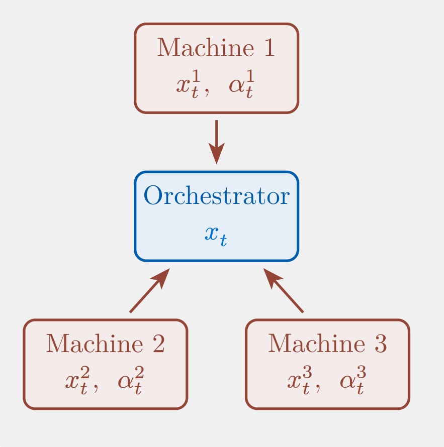
This decoupling introduces local replicas $x^j$, allowing workers to independently minimize local losses while the augmented quadratic penalty $\lambda |x^j - x|_2^2$ ensures global agreement and provides essential regularity for ill-conditioned or non-strongly convex functions. In this consensus mechanism, worker machines perform local refinement—balancing local fidelity with global consensus—while a central orchestrator aggregates these results to update the global variable $x$ via simple averaging.

Alternating Direction Method of Multipliers

The Alternating Direction Method of Multipliers (ADMM) is designed to solve convex optimization problems with separable objective functions of the form

, where $x \in \mathbb{R}^n, z \in \mathbb{R}^m, A \in \mathbb{R}^{p \times n}, B \in \mathbb{R}^{p \times m}$, and $c \in \mathbb{R}^p$ . The algorithm is constructed around the augmented Lagrangian,

ADMM can be interpreted as a strategic blend that inherits the decomposability of dual ascent and the superior convergence properties of the method of multipliers; crucially, instead of performing a joint minimization over primal variables, ADMM employs a single Gauss-Seidel pass that updates $x$ and $z$ sequentially . This alternating update consists of three steps:

To simplify these iterations, the linear and quadratic terms in the Lagrangian are combined by completing the square, defining a scaled dual variable $u := (1/\rho)\lambda$ such that

where $r$ is the residual $r := Ax + Bz - c$.

This transformation results in the scaled form of ADMM:

where $u^k$ effectively tracks the running sum of residuals $\sum_{j=1}^k r^j$.

In ADMM, primal residual is simply the constraint violation: \(r_{\text{prim}}^{k+1} := Ax^{k+1} + Bz^{k+1} - c.\)

Dual residual measures the gap to dual stationarity/consistency. Start from the first-order optimality condition (subgradient form) of the $x$-subproblem: \(0 \in \partial f(x^{k+1}) + A^\top y^k + \rho A^\top\bigl(Ax^{k+1} + Bz^k - c\bigr).\) Use the dual update to eliminate $y^k$: \(y^k = y^{k+1} - \rho\bigl(Ax^{k+1} + Bz^{k+1} - c\bigr) = y^{k+1} - \rho r_{\text{prim}}^{k+1}.\) Substituting back and rearranging (noting the difference between $z^k$ and $z^{k+1}$) gives \(0 \in \partial f(x^{k+1}) + A^\top y^{k+1} - \rho A^\top B\,(z^{k+1}-z^k).\) Since the KKT dual-stationarity condition is $0 \in \partial f(x^\star) + A^\top y^\star$, we define the dual residual as the deviation term: \(r_{\text{dual}}^{k+1} := \rho A^\top B\,(z^{k+1}-z^k).\)

General Convex QP with auxiliary variables and indicator functions

We start from general constrained trajectory optimization (the split/consensus form) with introducing an auxiliary variable $y$ as a general convex quadratic program.

, where $x\in\mathbb{R}^n$, $P\in\mathbb{S}_+^{n}$, $q\in\mathbb{R}^n$, $A\in\mathbb{R}^{m\times n}$, $b\in\mathbb{R}^m$ and a nonempty, closed, convex set $\mathcal{C}\subseteq\mathbb{R}^m$.

By introduction of auxiliary variables and consensus splitting with indicator functions

Introduce Lagrange multipliers $\lambda$ for $\tilde x-x=0$ and $\nu$ for $\tilde z-z=0$, with penalties $\sigma>0$ and $\rho>0$. The (unscaled) augmented Lagrangian is

Complete the square for the $\tilde x=x$ and $\tilde z=z$ coupling term:

For $\arg\min$ steps in ADMM, the constants $-\frac{1}{2\sigma}|\lambda|_2^2$ and $-\frac{1}{2\rho}|\nu|_2^2$ can be dropped. This yields a scaled-penalty form where $\lambda$ and $\nu$ appear only through $\sigma^{-1}\lambda$ and $\rho^{-1}\nu$.

Finally

OSQP as an operator splitting solver

Use two-block ADMM with block 1: $(\tilde x,\tilde z)$ and block 2: $(x,z)$. Each following step involves fixing other variables and minimizing/maximizing the current variable.

Fix $(x^k,z^k,\lambda^k,\nu^k)$ and update $(\tilde x,\tilde z)$ by minimizing the scaled augmented Lagrangian over $(\tilde x,\tilde z)$ ([2] eq.15):

We get the pair $(\tilde x^{k+1},\tilde z^{k+1})$, the linear–quadratic core with a consensus proximal term, it solves a quadratically regularized subproblem that enforces the linear equality $A\tilde x=\tilde z$ while minimizing $\tfrac12\tilde x^\top P\tilde x+q^\top\tilde x$, and is pulled toward the previous iterate $(x^k,z^k)$ via the penalties $\tfrac{\sigma}{2}|\tilde x-x^k+\sigma^{-1}\lambda^k|_2^2+\tfrac{\rho}{2}|\tilde z-z^k+\rho^{-1}\nu^k|_2^2$.

The variables $(x^{k+1},z^{k+1})$ in following are obtained by proximal steps for the constraint/indicator terms ($z^{k+1}=\Pi_{\mathcal C}(\hat z^{k+1}+\rho^{-1}\nu^k)$), and over-relaxation uses the extrapolated point $\hat z^{k+1}=\alpha\tilde z^{k+1}+(1-\alpha)z^k$ ($\alpha>1$) so that the argument of the projection is pushed closer to the “correct side” of the constraint set, often reducing zig-zagging and accelerating convergence. (Similar to Mehrotra Predictor Corrector)

Fix $(\tilde x^{k+1},\tilde z^{k+1},z^k,\lambda^k,\nu^k)$ and update $x$ by minimizing the $x$-dependent term:

The minimizer satisfies $\hat x^{k+1}-x^{k+1}+\sigma^{-1}\lambda^k=0$, hence ([2] eq.16)

Fix $(\tilde z^{k+1},x^{k+1},\nu^k)$ and update $z$ by minimizing the $z$-dependent terms as a proximal mapping::

Since $\mathcal{I}_{\mathcal C}$ is the indicator function of $\mathcal C$, its proximal mapping coincides with the Euclidean projection onto $\mathcal C$, hence

Update the dual variables by gradient ascent on the coupling constraints: ([2] eq.18, 19)

From $\hat x^{k+1}-x^{k+1}=-\sigma^{-1}\lambda^k$, hence

so $\lambda^{k+1}=0$ for all $k\ge 0$.

Computational Core of OSQP and its numerical implementation

Everything is cheap in ADMM except the $(\tilde x,\tilde z)$-subproblem~(★). In OSQP, (★) is an equality-constrained quadratic program—quadratic objective in $(\tilde x,\tilde z)$ with an affine constraint $A\tilde x=\tilde z$—so its first-order optimality conditions reduce to a sparse KKT linear system.([1] §4.2.5)

Moreover, the $\tilde x=x$ multiplier vanishes identically: from $x^{k+1}=\hat x^{k+1}+\sigma^{-1}\lambda^k$ and $\lambda^{k+1}=\lambda^k+\sigma(\hat x^{k+1}-x^{k+1})$ we get $\lambda^{k+1}=0$. With the natural initialization $\lambda^0=0$, this implies $\lambda^k\equiv 0$ for all $k$. Hence, in the computational core below we can drop the shift $\sigma^{-1}\lambda^k$ in~(★), the $\sigma$-penalty contributes simply $\frac{\sigma}{2}|\tilde x-x^k|_2^2$.

Writing the Lagrangian of (★) with multiplier $\gamma^{k+1}$ for the constraint $A\tilde x=\tilde z$, the KKT conditions are:

where $\nu^k$ is the ADMM dual iterate associated with $\tilde z=z$. Eliminating $\tilde z^{k+1}$ yields the $2\times 2$ block KKT system:

The resulting KKT matrix is always full rank (the subproblem is always solvable) thanks to consensus regularizers $\sigma>0$ and $\rho>0$, without requiring strong convexity or constraint independence.

The following ideas form a practical implementation checklist for solving this sparse KKT linear system:

• Direct solve (factorization + back-solve):
  Treat the KKT matrix as fixed (or slowly changing) and compute a sparse factorization once, e.g.,

  \[K \approx LDL^\top,\]

  where $L$ is sparse and $D$ is (block) diagonal. Then each ADMM iteration only requires cheap forward/backward substitutions (triangular solves) to recover $\tilde x^{k+1}$ and the associated multipliers.
  Intuition: factorization is the expensive part; back-solves are much cheaper.

• Exploit sparsity (permutation + sparse linear algebra):
  The KKT matrix is typically sparse (because $P$ and $A$ are sparse). A naive factorization can create many “fill-in” nonzeros and become slow or memory-heavy. The remedy is to reorder variables with a permutation $ \Pi $ and factorize

  \[\Pi K \Pi^\top = LDL^\top,\]

  choosing $ \Pi $ to reduce fill-in. In practice, one also separates symbolic factorization (analyzing the sparsity pattern and deciding the fill-in structure) from numeric factorization (computing the actual values).
  Intuition: the ordering determines whether a sparse problem stays sparse during factorization.

• Cache the factorization (amortize the expensive step):
  ADMM needs many iterations. If the coefficient matrix $K$ is unchanged across iterations, we should reuse the same $LDL^\top$ every time. That means: do the factorization once, then do only the back-solves each iteration. If $K$ changes occasionally (e.g., when penalty parameters change), we refactorize only at those events.
  Intuition: pay the “one-time” cost once, then enjoy cheap iterations.

• Indirect solve (elimination + iterative method, enabling inexact minimization):
  When the problem is very large, even sparse factorization can be too expensive (memory or time). An alternative is to eliminate variables to obtain an equivalent symmetric positive definite (SPD) system of the form

  \[(P+\sigma I+\rho A^\top A)\,\tilde x = \text{rhs},\]

  and solve it with an iterative Krylov method such as Conjugate Gradient (CG). Crucially, CG can be truncated: we stop once the linear residual is below a chosen tolerance, rather than solving to machine precision. This is exactly how “inexact subproblem solves” appear in practice: early ADMM iterations can use coarse CG tolerances, while later iterations tighten them if higher accuracy is needed.
  Intuition: replace a heavy one-shot factorization with many cheap matrix-vector products, and allow approximate solves when exactness is not worth the cost.

Inexact minimization ([1] §3.4.4) as indirect CG truncation in OSQP:

instead of solving (★) exactly, CG is stopped once the linear system residual is below a prescribed tolerance. [1] explicitly justifies early termination of iterative inner solvers using convergence results for ADMM with inexact minimization, recommending low accuracy in early ADMM iterations and gradually increasing it, plus warm starting the inner solver.

$\rho$ selection: From Residual Balancing to Solver-Grade Heuristics

While the KKT system provides the search direction, the practical convergence speed of ADMM hinges on a single numerical knob: the step-size parameters $\sigma$ and, most critically, augmented Lagrangian penalty $\rho$. In the scaled ADMM form derived above, $\rho$ determines the step-size of the dual variable update.

The optimality conditions require both the primal residual $r_{\text{prim}}$ (constraint violation) and dual residual $r_{\text{dual}}$ (optimality violation) to vanish.If $\rho$ is large, the penalty on infeasibility is heavy; $r_{\text{prim}}$ decreases quickly, but the dual problem becomes stiff.If $\rho$ is small, the algorithm is “gentler” on feasibility; $r_{\text{dual}}$ decreases quickly, but primal constraints may be violated for longer. [1] 3.4.1 Varying Penalty Parameter employs a scalar $\rho$ with a simple feedback loop: increase $\rho$ if $|r_{\text{prim}}| \gg |r_{\text{dual}}|$ and decrease it if $|r_{\text{dual}}| \gg |r_{\text{prim}}|$.

OSQP departs from the scalar parameter approach by treating $\rho$ as a positive definite diagonal matrix $\rho \in \mathbb{S}_{++}^m$. This allows the solver to assign different penalties to different constraints, effectively “preconditioning” the problem based on constraint type.The “Oracle” Intuition: If we knew the active set at optimality a priori, we would set $\rho_i \to \infty$ for active constraints (enforcing them as equalities) and $\rho_i \to 0$ for inactive constraints (ignoring them).Initialization Heuristic: Since the active set is unknown, OSQP initializes $\rho$ based on the problem structure. For strict equality constraints (where $l_i = u_i$), it sets a high penalty ($\rho_i = 10^3 \bar{\rho}$) to approximate the “active” behavior, while inequality constraints use a lower default $\bar{\rho}$.

Dynamic updates introduce a critical engineering constraint. The KKT matrix $K(\rho)$ depends explicitly on $\rho$ in its $(2,2)$-block:

Since changing $\rho$ invalidates the cached $LDL^\top$ factorization of $K$, OSQP employs a conservative trigger policy. The parameter is updated only if:

Metric: It computes the update factor based on the square root of the ratio of scaled residuals. The imbalance is significant (based on scaled residuals):

Trigger: The computational investment is justified:

(accumulated iteration time exceeds 40% of the factorization time) This ensures the solver only pays the “refactorization penalty” when the numerical benefits clearly outweigh the CPU cost.

Optimality & Stopping Criteria

A step $k$ we measure the distance from the destination using residuals:

Standard implementations often rely on a single scalar tolerance $\epsilon$, requiring $|r|_2 \le \epsilon$. However, this is numerically fragile: the condition becomes practically impossible to satisfy if the problem data (the “signal”) is much larger than 1, yet becomes dangerously loose if the signal is much smaller than 1.

To build a robust solver, OSQP makes two critical engineering upgrades : It uses the infinity norm $\lVert \cdot \rVert_\infty$ to ensure that the worst-case violation of any single constraint is bounded. Tolerances are decomposed into an absolute part $\epsilon_{\text{abs}}$ and a relative part $\epsilon_{\text{rel}}$, scaled by the magnitude of the current iterates.

This ensures that the error is always judged relative to the signal magnitude flowing through the system, allowing OSQP to handle problem scales ranging from micro-robotics to massive infrastructure models without manual retuning.

Result for simple QP

Under standard regularity assumptions, strong convexity and smoothness of the quadratic objective and full column rank of the constraint operator, ADMM achieves a global linear convergence rate on this QP,

[ code →]

Future work

Preconditioning, Infeasibility Detection and Solution Polishing in OSQP is valuable to explore in the future. Same method for conic optimization (SCS solver) [3] can be explored in the future.

References

[1] S. Boyd, N. Parikh, E. Chu, B. Peleato, J. Eckstein, et al., “Distributed optimization and statistical learning via the alternating direction method of multipliers,” Foundations and Trends® in Machine learning, vol. 3, no. 1, pp. 1–122, 2011.

[2] B. Stellato, G. Banjac, P. Goulart, A. Bemporad, and S. Boyd, “Osqp: An operator splitting solver for quadratic programs,” Mathematical Programming Computation, vol. 12, no. 4, pp. 637–672, 2020.

[3] B. O’donoghue, E. Chu, N. Parikh, and S. Boyd, “Conic optimization via operator splitting and homogeneous self-dual embedding,” Journal of Optimization Theory and Applications, vol. 169, pp. 1042–1068, 2016.

[4] G. Farina, “Lecture 16: Distributed optimization and ADMM,” MIT 6.7220 / 15.084 Nonlinear Optimization, Spring 2025, MIT, Lecture notes. [Online]. https://www.mit.edu/~gfarina/2025/67220s25_L16_admm/L16.pdf