Infeasible-start Mehrotra’s Predictor-Corrector IPM
Reproducing the CVXGEN/qpSWIFT/HPIPM Algorithm Logic from scratch
TL;DR
Infeasible-start Mehrotra’s predictor–corrector method is one of the most effective primal–dual interior-point schemes for convex QPs, this project rebuilt the method from first principles, with emphasis on what makes it work in practice: affine prediction, adaptive centering/correction, positivity-preserving step control, strictly interior initialization, and practical safeguards for positivity and residual reduction. Beyond implementation, the project clarifies the algorithmic logic that makes Mehrotra’s method both more aggressive and more robust than a plain Newton-step PD-IPM or a classic predictor–corrector method.
Problem setup
This project solves Quadratic Programs, with the log-barrier subproblem for the slack variables $s$ with fixed $t >0$:
\[\begin{array}{@{}l@{\qquad}c@{\qquad}l@{}} \begin{aligned} \min_{x\in\mathbb R^n}\quad & \frac12 x^\top Qx + q^\top x \\ \text{s.t.}\quad & Ax=b \\ & Gx \le h \end{aligned} & \Longrightarrow & \begin{aligned} \min_{\{x,s\}\in\mathbb R^{n+m}}\quad & \frac12 x^\top Qx + q^\top x - \frac{1}{t}\sum_{i=1}^{m}\log s_i \\ \text{s.t.}\quad & Gx + s = h\\ & Ax = b \end{aligned} \end{array}\], where $Q\succeq 0$, $A\in\mathbb R^{p\times n}$, $G\in\mathbb R^{m\times n}$, $b\in\mathbb R^{p}$, $h,s\in\mathbb R^{m}$.
The Modified KKT system for barrier subproblem:
\[\begin{cases} Qx + q + G^\top \lambda + A^\top \nu = 0,\\ {s_i}\lambda_i = \frac{1}{t} \quad \forall i = 1,\cdots, m,\\ Gx+s-h=0,\\ Ax-b=0, \end{cases} \qquad \text{with } s\succ 0,\ \lambda \succ 0.\]write as the residual vector:
\[r_t(x,s,\lambda,\nu) = \begin{bmatrix} r_{\mathrm{dual}}\\ r_{\mathrm{cent}}\\ r_{\mathrm{pri,ineq}}\\ r_{\mathrm{pri,eq}} \end{bmatrix} := \begin{bmatrix} Qx + q + G^\top\lambda + A^\top\nu\\ \operatorname{diag}(s)\lambda - \tfrac{1}{t}\mathbf 1\\ Gx + s - h\\ Ax - b \end{bmatrix}.\]Let the stacked variable be $ \mathcal{X} := [\,x,\; s,\; \lambda,\; \nu\,]^{\top}$. A Newton step search direction at current $\mathcal{X}$ by solving $ D r_t(\mathcal{X})\,\Delta \mathcal{X} = - r_t(\mathcal{X})$, explicitly:
\[\begin{bmatrix} Q & 0 & G^\top & A^\top\\ 0 & \operatorname{diag}(\lambda) & \operatorname{diag}(s) & 0\\ G & I & 0 & 0\\ A & 0 & 0 & 0 \end{bmatrix} \begin{bmatrix} \Delta x\\ \Delta s\\ \Delta\lambda\\ \Delta\nu \end{bmatrix} = - \begin{bmatrix} r_{\mathrm{dual}}\\ r_{\mathrm{cent}}\\ r_{\mathrm{pri,ineq}}\\ r_{\mathrm{pri,eq}} \end{bmatrix}.\]In the primal-dual interior-point method, the iterates $\mathcal{X}^{(k)} = [x^{(k)}, s^{(k)},\lambda^{(k)}, \nu^{(k)}]^{\top}$ are not necessarily feasible, except in the limit as the algorithm converges. Surrogate duality gap was used to evaluate duality gap. The surrogate duality gap and average complementarity defined as
\[\hat\eta := s^\top \lambda = \sum_{i=1}^{m} s_i\lambda_i, \quad \bar\eta := \frac{\hat\eta}{m}=\frac{s^\top \lambda}{m}.\]Along the central path for fixed $t$, surrogate duality gap become $\hat\eta = \sum_{i=1}^{m}1/t = m/t.$
Standard Primal–dual interior-point method for this QP
The original method chooses $t$ from the current iterate via $\hat\eta$, computes one primal–dual Newton direction for $r_t(\mathcal{X})=0$, then performs a backtracking line search to update $\mathcal{X}$.
Since near the central path $\hat\eta\approx m/t$, the update targets a reduction of the gap scale by roughly a scaling factor $\mu$ (increases $t$ by $\mu$ when near centrality). Given current $\hat\eta=s^\top\lambda$, set
\[t^{+} := \mu \frac{m}{\hat\eta}=\mu t, \qquad \mu>1\]And the method terminate when:
\[\lVert r_{\mathrm{pri}}\rVert_2 \le \epsilon_{\mathrm{feas}},\ \lVert r_{\mathrm{dual}}\rVert_2 \le \epsilon_{\mathrm{feas}},\ \hat\eta \le \epsilon.\]After computing $\Delta \mathcal{X}$ from newton step, update $\mathcal{X}^+ = x + \alpha \Delta \mathcal{X}$ with step length $\alpha\in(0,1]$ chosen by backtracking.
In order to maintain interior feasibility (domain constraints), we must keep $s^+ \succ 0,\quad \lambda^+ \succ 0.$ Compute the maximum allowable step (not exceeding 1), and initialize $\alpha \leftarrow 0.99\,\alpha_{\max}$:
\[\alpha_{\max}=\min\Bigl( 1,\ \min_{i:\Delta s_i<0}\Bigl(-\frac{s_i}{\Delta s_i}\Bigr),\ \min_{i:\Delta\lambda_i<0}\Bigl(-\frac{\lambda_i}{\Delta\lambda_i}\Bigr) \Bigr).\]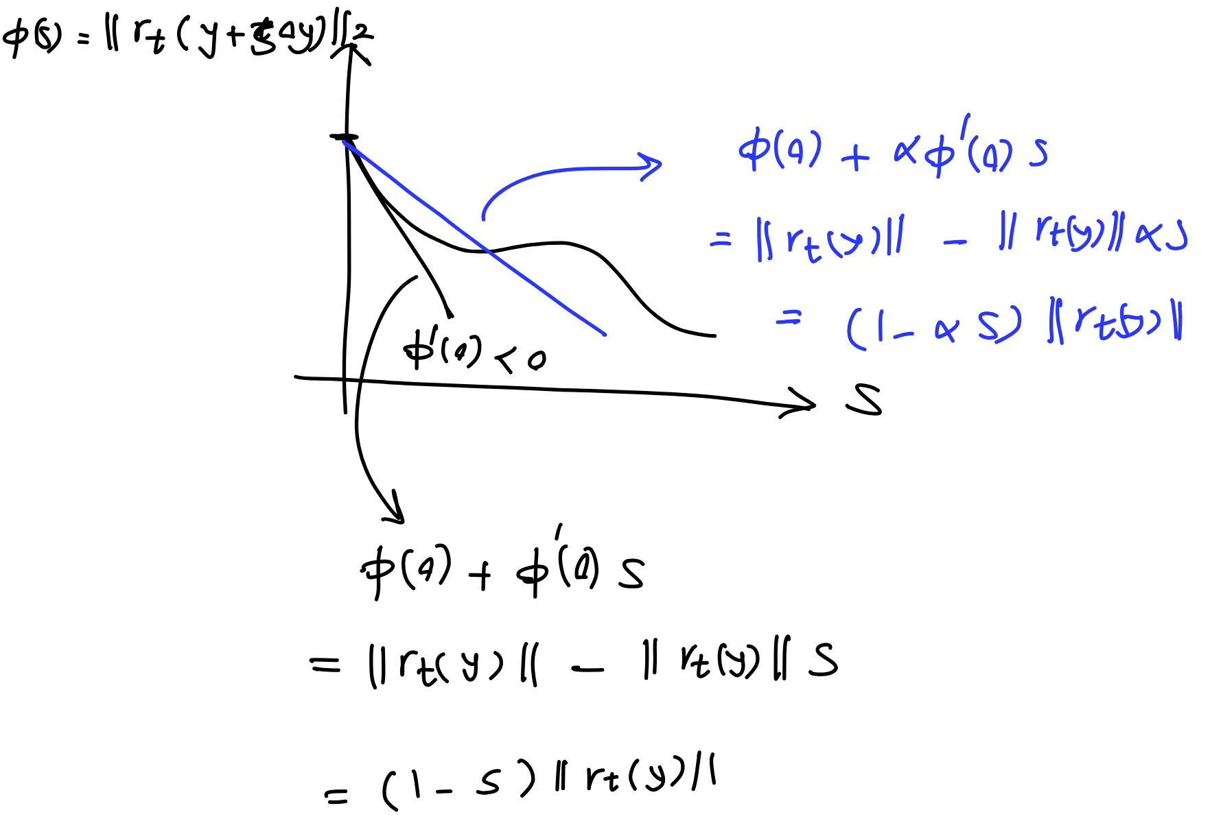
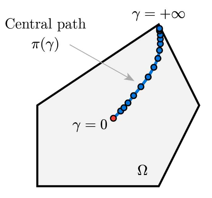
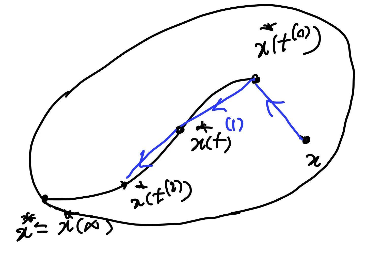
Tangent to central path
We consider the central path $x^\star(t) = \arg\min_{x}\; t f_0(x) + \phi(x),$ which, by optimality, satisfies the centrality (stationarity) equation $t \nabla f_0\bigl(x^\star(t)\bigr) + \nabla \phi\bigl(x^\star(t)\bigr) = 0.$
Viewing this equation as an implicit definition of $x^\star(t)$ as a function of $t$, implicit differentiation with respect to $t$ yields the tangent direction along the central path:
\[\frac{d x^\star(t)}{d t} = -\Bigl(t \nabla^2 f_0\bigl(x^\star(t)\bigr) + \nabla^2 \phi\bigl(x^\star(t)\bigr)\Bigr)^{-1} \nabla f_0\bigl(x^\star(t)\bigr).\]Consequently, the first-order predictor obtained by increasing $t$ from $t$ to $\mu t$ is
\[\hat{x} = x^\star(t) + \frac{d x^\star(t)}{d t}(\mu t - t)\]which simply approximates $x^\star(\mu t)$ by moving along the tangent of the central path.
Since we use surrogate duality gap to evaluate duality gap, $\hat{\eta} = s^\top \lambda$ and $\bar{\eta} = \hat{\eta}/m$, a more natural way is to treat central path and decision variable as implicit functions of $\bar{\eta}$ and use tangent line as predictor
\[\mathcal{X}(\bar{\eta}^+) \approx \mathcal{X}(\bar{\eta}) + \frac{d \mathcal{X}^\star}{d \bar{\eta}} \bigl(\bar{\eta}^+ - \bar{\eta}\bigr).\]On the central path, $s_i \lambda_i = 1/t$, therefore $\bar{\eta} = 1/t$. Hence, $t^+ = \mu t \Longleftrightarrow \bar{\eta}^+ = \bar{\eta}/\mu$. That is the outer update rather driving down the gap scale $\bar{\eta}$. We write the central path as an implicit equation parameterized by $\bar{\eta}$:
\[r(x,s,\lambda,\nu;\bar{\eta}) = \begin{bmatrix} r_{\mathrm{dual}} \\ r_{\mathrm{cent}}(\bar{\eta}) \\ r_{\mathrm{pri,ineq}} \\ r_{\mathrm{pri,eq}} \end{bmatrix} = \begin{bmatrix} Qx + q + G^\top \lambda + A^\top \nu \\ \mathrm{diag}(s)\lambda - \bar{\eta}\mathbf{1} \\ Gx + s - h \\ Ax - b \end{bmatrix} = 0.\]Differentiate $r(\mathcal{X}^\star;\bar{\eta}) = 0$ with respect to $\bar{\eta}$ using implicit function theorem:
\[D_{\mathcal{X}} r(\mathcal{X};\bar{\eta})\,\frac{d\mathcal{X}^\star(\bar{\eta})}{d\bar{\eta}} + \frac{\partial r}{\partial \bar{\eta}} = 0.\]Note that only $r_{\mathrm{cent}}$ depends on $\bar{\eta}$, so $\partial r/\partial \bar{\eta}=[0,-\mathbf{1},0,0]^{\top}$. $D_{\mathcal{X}} r$ is the KKT Jacobian block above, and tangent vector satisfy :
\[D_{\mathcal{X}} r= \begin{bmatrix} Q & 0 & G^\top & A^\top\\ 0 & \operatorname{diag}(\lambda) & \operatorname{diag}(s) & 0\\ G & I & 0 & 0\\ A & 0 & 0 & 0 \end{bmatrix}, \quad D_{\mathcal{X}} r \cdot\frac{d\mathcal{X}^\star(\bar{\eta})}{d\bar{\eta}}=\begin{bmatrix} 0\\ \mathbf{1}\\ 0\\ 0 \end{bmatrix}\]From the Tangent to the Affine-Scaling Predictor: Mehrotra’s First Step
Now let’s first construct an aggressive predictor by setting an extreme target: take the next step directly to $\bar{\eta}^{+}=0$ , drive the average complementarity directly to zero, reduce the complementarity without any explicit centering.
If the current point is near the central path:$r_{\mathrm{dual}} \approx r_{\mathrm{pri}} \approx 0,\quad \mathrm{diag}(s)\lambda \approx \bar{\eta}\mathbf{1}.$
Then the tangent step corresponding to pushing $\bar{\eta}$ from its current value to $0$ is simply
\[\Delta\bar{\eta} = -\bar{\eta}.\]Plugging into the tangent equation gives (on the central path, $\bar{\eta}\mathbf{1}=\mathrm{diag}(s)\lambda$):
\[\begin{bmatrix} Q & 0 & G^\top & A^\top\\ 0 & \operatorname{diag}(\lambda) & \operatorname{diag}(s) & 0\\ G & I & 0 & 0\\ A & 0 & 0 & 0 \end{bmatrix}\,\Delta\mathcal{X} = \begin{bmatrix} 0\\ 1\\ 0\\ 0 \end{bmatrix}\Delta\bar{\eta} = \begin{bmatrix} 0\\ -\bar{\eta}\mathbf{1}\\ 0\\ 0 \end{bmatrix} = \begin{bmatrix} 0\\ -\mathrm{diag}(s)\lambda\\ 0\\ 0 \end{bmatrix} = \begin{bmatrix} 0\\ -\,s\circ\lambda\\ 0\\ 0 \end{bmatrix}.\]This explains why Mehrotra Step uses $-\mathrm{diag}(s)\lambda$ in Mehrotra’s first (Newton-like) step: it is the direction that predicts along the central-path tangent pushing $\bar{\eta}$ toward $0$ (and it matches exactly on the central path).
Away from the central path, we must simultaneously reduce the primal and dual residuals $r_{\mathrm{dual}}, r_{\mathrm{pri}}$ simultaneously, so the affine predictor actually solves the linear system:
\[\begin{bmatrix} Q & 0 & G^\top & A^\top\\ 0 & \operatorname{diag}(\lambda) & \operatorname{diag}(s) & 0\\ G & I & 0 & 0\\ A & 0 & 0 & 0 \end{bmatrix} \begin{bmatrix} \Delta x^{\mathrm{aff}}\\ \Delta s^{\mathrm{aff}}\\ \Delta \lambda^{\mathrm{aff}}\\ \Delta \nu^{\mathrm{aff}} \end{bmatrix} = - \begin{bmatrix} r_{\mathrm{dual}}\\ \mathrm{diag}(s)\lambda\\ r_{\mathrm{pri,ineq}}\\ r_{\mathrm{pri,eq}} \end{bmatrix}.\]Line search for affine-scaling predictor is exactly same as the one for original newton step:
\[\alpha^{\mathrm{aff}} \leftarrow 0.99\,\alpha_{\max}^{\mathrm{aff}}, \quad \alpha_{\max}^{\mathrm{aff}} = \min\Bigl( 1,\ \min_{i:\Delta s^{\mathrm{aff}}_i<0}\Bigl(-\frac{s_i}{\Delta s^{\mathrm{aff}}_i}\Bigr),\ \min_{i:\Delta\lambda^{\mathrm{aff}}_i<0}\Bigl(-\frac{\lambda_i}{\Delta\lambda^{\mathrm{aff}}_i}\Bigr) \Bigr).\]So the predicted surrogate duality gap at the affine step is:
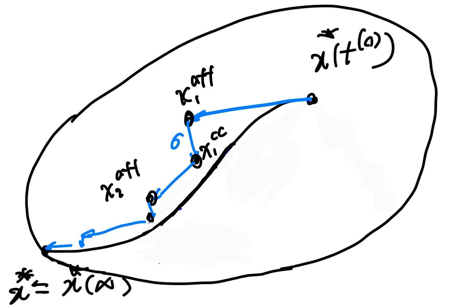
\[\hat{\eta}^{\mathrm{aff}} := \bigl(s+\alpha^{\mathrm{aff}}\Delta s^{\mathrm{aff}}\bigr)^\top \bigl(\lambda+\alpha^{\mathrm{aff}}\Delta \lambda^{\mathrm{aff}}\bigr), \quad \bar{\eta}^{\mathrm{aff}} := \frac{\hat{\eta}^{\mathrm{aff}}}{m}.\]Second Step: Centering-plus-corrector Directions
Mehrotra’s second step uses the affine predictor to choose an adaptive centering strength:
\[\sigma = \left(\frac{\hat{\eta}^{\mathrm{aff}}}{\hat{\eta}}\right)^3 = \left( \frac{\bigl(s+\alpha^{\mathrm{aff}}\Delta s^{\mathrm{aff}}\bigr)^\top \bigl(\lambda+\alpha^{\mathrm{aff}}\Delta \lambda^{\mathrm{aff}}\bigr)} {s^\top \lambda} \right)^{3} ,\]to adaptively decide how much “centering” to enforce in the next step (Or $\sigma$ can be set by heuristic, smaller $\sigma$ is more aggressive; larger $\sigma$ is more conservative, pulling harder back toward the center).This changes a key point of original PD-IPM: we originally hand-fixed the outer growth factor $\mu$; Mehrotra uses the affine predictor to automatically estimate how small it can drive $\bar{\eta}$, and then backs out an appropriate centering strength $\sigma$.
Therefore the new centering target we want (componentwise) is
\[s_i^{+}\lambda_i^{+} \approx \sigma\bar{\eta},\quad i=1,\ldots,m, \quad (s+\Delta s)\circ(\lambda+\Delta\lambda)\approx \sigma\bar{\eta}\mathbf{1}\]Expanding elementwise gives
\[s\circ\lambda +\mathrm{diag}(s)\Delta\lambda +\mathrm{diag}(\lambda)\Delta s +(\Delta s\circ\Delta\lambda) =\sigma\bar{\eta}\mathbf{1}.\]A standard Newton linearization drops the second-order term $\Delta s\circ\Delta\lambda$: $\mathrm{diag}(s)\Delta\lambda +\mathrm{diag}(\lambda)\Delta s =\sigma\bar{\eta}\mathbf{1}-s\circ\lambda.$ The affine predictor corresponds exactly to this linearized equation with $\sigma=0$: $ \mathrm{diag}(s)\Delta\lambda^{\mathrm{aff}} +\mathrm{diag}(\lambda)\Delta s^{\mathrm{aff}} =-\,s\circ\lambda.$
Although the affine predictor makes the linearized complementarity residual small, the true complementarity at the affine step contains the quadratic term $\Delta s^{\mathrm{aff}}\circ\Delta\lambda^{\mathrm{aff}}$, which can be large and typically pushes the iterates toward the boundary. The corrector modifies the complementarity equation by (i) shifting the target from $0$ to $\sigma\bar{\eta}\mathbf{1}$ (centering) $ \mathrm{diag}(s)\Delta\lambda^{\mathrm{cc}} +\mathrm{diag}(\lambda)\Delta s^{\mathrm{cc}} =\sigma\bar{\eta}\mathbf{1}. $
and (ii) subtracting the estimated quadratic error (corrector) $\Delta s\circ\Delta\lambda\approx\Delta s^{\mathrm{aff}}\circ\Delta\lambda^{\mathrm{aff}}.$
Therefore, plug into $s\circ\lambda+\mathrm{diag}(s)\Delta\lambda+\mathrm{diag}(\lambda)\Delta s+(\Delta s\circ\Delta\lambda)=\sigma\bar{\eta}\mathbf{1},\; \mathrm{diag}(s)\Delta\lambda^{\mathrm{aff}} +\mathrm{diag}(\lambda)\Delta s^{\mathrm{aff}} =-\,s\circ\lambda,$ the centering block in the corrector becomes
\[\mathrm{diag}(s)\Delta\lambda^{\mathrm{cc}} +\mathrm{diag}(\lambda)\Delta s^{\mathrm{cc}} = \sigma\bar{\eta}\mathbf{1} - \bigl(\Delta s^{\mathrm{aff}}\circ\Delta\lambda^{\mathrm{aff}}\bigr).\]So the centering-plus-corrector directions solves linear system
\[\begin{bmatrix} Q & 0 & G^\top & A^\top\\ 0 & \operatorname{diag}(\lambda) & \operatorname{diag}(s) & 0\\ G & I & 0 & 0\\ A & 0 & 0 & 0 \end{bmatrix} \begin{bmatrix} \Delta x^{\mathrm{cc}}\\ \Delta s^{\mathrm{cc}}\\ \Delta\lambda^{\mathrm{cc}}\\ \Delta\nu^{\mathrm{cc}} \end{bmatrix} = \begin{bmatrix} 0\\ \sigma\bar{\eta}\mathbf{1} - \mathrm{diag}(\Delta s^{\mathrm{aff}})\Delta\lambda^{\mathrm{aff}}\\ 0\\ 0 \end{bmatrix}.\]The final combined search direction is then $\Delta\mathcal X=\Delta\mathcal X^{\mathrm{aff}}+\Delta\mathcal X^{\mathrm{cc}},$ explcitly conbime two direction vectors:
\[\begin{bmatrix} \Delta x \\ \Delta s \\ \Delta \lambda \\ \Delta \nu \end{bmatrix} = \begin{bmatrix} \Delta x^{\mathrm{aff}} \\ \Delta s^{\mathrm{aff}} \\ \Delta \lambda^{\mathrm{aff}} \\ \Delta \nu^{\mathrm{aff}} \end{bmatrix} + \begin{bmatrix} \Delta x^{\mathrm{cc}} \\ \Delta s^{\mathrm{cc}} \\ \Delta \lambda^{\mathrm{cc}} \\ \Delta \nu^{\mathrm{cc}} \end{bmatrix}.\]Given $\Delta\mathcal X$, line search is same as previous enforcing interior feasibility, explicitly
\[\alpha = \min\left\{ 1,\; 0.99 \sup\left\{ \alpha \ge 0 \ \middle|\ s + \alpha\,\Delta s \ge 0,\ \lambda + \alpha\,\Delta \lambda \ge 0 \right\} \right\}.\]Now update the primal and dual variables $\mathcal X^{+}=\mathcal X+\alpha\,\Delta\mathcal X$.
Initialization
Following [5] Section 5 Path-following algorithm for cone QPs, primal and dual starting points are selected as follows:
Here solve the analytical solution for the primal problem:
\[\begin{aligned} \min_{x,s}\quad & \frac{1}{2}x^\top Qx + q^\top x + \frac{1}{2}\|s\|_2^2\\ \text{s.t.}\quad & Gx + s = h,\\ & Ax = b, \end{aligned}\]which can be written as the block system
\[\begin{bmatrix} Q & G^\top & A^\top\\ G & -I & 0\\ A & 0 & 0 \end{bmatrix} \begin{bmatrix} x\\ \lambda\\ \nu \end{bmatrix} = \begin{bmatrix} -q\\ h\\ b \end{bmatrix}.\]The dual problem is
\[\begin{aligned} \max_{w,\lambda,\nu}\quad & -\frac{1}{2}w^\top Qw - h^\top \lambda - b^\top \nu - \frac{1}{2}\|\lambda\|_2^2\\ \text{s.t.}\quad & Qw + q + G^\top \lambda + A^\top \nu = 0. \end{aligned}\]This initialization solves a different, regularized primal–dual pair and serves as a generic, numerically stable way to generate a strictly interior starting point. The added norm terms tend to keep the slack magnitude moderate—so the implied inequality violation as measured by $\lVert s \rVert_2^2,\lVert \lambda \rVert_2^2$ in primal-dual problem is typically not extreme—but the construction is not intended to provide a starting point that is necessarily close to the optimal solution.
Now shift the linear system solution to a strictly interior starting point. After solving the regularized equality-constrained system to obtain provisional $(x^{(0)},\nu^{(0)})$, we form the inequality residual
\[r := Gx^{(0)} - h\]Define the minimum shifts that make the slack and multiplier nonnegative componentwise:
\[\alpha_p := \inf\{\alpha\in\mathbb{R}\mid -r + \alpha \mathbf{1} \ge \mathbf{0}\},\qquad \alpha_d := \inf\{\alpha\in\mathbb{R}\mid \;\;r + \alpha \mathbf{1} \ge \mathbf{0}\}.\]then set
\[s^{(0)} := \begin{cases} -r, & \alpha_p < 0,\\ -r + (1+\alpha_p)\mathbf{1}, & \text{otherwise}, \end{cases} \qquad \lambda^{(0)} := \begin{cases} r, & \alpha_d < 0,\\ r + (1+\alpha_d)\mathbf{1}, & \text{otherwise}. \end{cases}\]This simple shift guarantees a strictly interior initialization $s^{(0)}>\mathbf{0}$ and $\lambda^{(0)}>\mathbf{0}$, yielding the starting point $\mathcal{X}^{(0)} := \bigl[x^{(0)},\, s^{(0)},\, \lambda^{(0)},\, \nu^{(0)}\bigr]^\top$.
At each iteration,
1) check termination based on primal/dual residual norms and the surrogate duality gap;
2) compute an affine-scaling predictor search direction.
3) compute a centering-plus-corrector direction;
4) backtracking line search in residuals;
5) update the primal and dual variables and repeat.
Result for simple QP


Future work
Nearly all of the computational effort is in the solution of the linear systems in steps 2 and 3 which detailed introduced above. Both linear systems have same LHS with same structured KKT matrix. Numerical factorization can be futher explored.
References
[1]. Boyd, S. & Vandenberghe, L. Convex Optimization. Cambridge University Press, 2004.
[2]. Mattingley, J. & Boyd, S. CVXGEN: a code generator for embedded convex optimization, Optimization and Engineering, vol. 13, no. 1, pp. 1-27, 2012.
[3]. Pandala, A. G., Ding, Y., & Park, H.-W. qpSWIFT: A Real-Time Sparse Quadratic Program Solver for Robotic Applications, IEEE Robotics and Automation Letters, vol. 4, no. 4, pp. 3355–3362, Oct. 2019. doi:10.1109/LRA.2019.2926664
[4]. Mehrotra, S. On the Implementation of a Primal-Dual Interior Point Method, SIAM Journal on Optimization, vol. 2, no. 4, pp. 575–601, 1992. doi:10.1137/0802028
[5]. Vandenberghe, L. The CVXOPT linear and quadratic cone program solvers. Technical report / notes, March 20, 2010. https://www.seas.ucla.edu/~vandenbe/publications/coneprog.pdf