Model-Based Fixed-Wing Perching
TL;DR
Fixed-wing perching is a canonical underactuated control problem: a small glider must enter a strongly nonlinear post-stall regime, generate enough drag to stop quickly, and still hit a tiny perch. This project rebuilds the model-based pipeline behind that behavior: a flat-plate physics prior, data-driven aerodynamic residuals, online calibration, trajectory optimization, TVLQR stabilization, funnel analysis, and sampling-based alternatives such as MPPI and CEM. The central lesson is that the model does not need to be perfect; it needs to be structured enough for planning and feedback to reason through the maneuver.
One of my favorite case studies in Underactuated Robotics asks a wonderfully simple question:
Can a fixed-wing aircraft land on a perch the way a bird does?
A conventional aircraft is designed to avoid stall: keep the flow attached, dissipate energy gradually, and ask for a runway. A perching bird does almost the opposite. It pitches up, enters a post-stall regime, creates enormous drag, and still lands precisely.
That is what makes fixed-wing perching beautiful. The problem is not simply to slow down; it is to slow down aggressively while preserving enough control authority to hit a small target. To isolate that difficulty, Russ’s group stripped the system down to a planar glider: no propeller, flat-plate wings, one actuated tail, and enough dihedral to make roll mostly passive. The input is just
\[u=\dot\phi .\]A flat plate is a terrible high-performance airfoil, which is exactly why it is useful here. Perching lives at large angle of attack, where attached-flow intuition breaks down. We want a model that captures the dominant post-stall force scaling, not one that pretends every vortex is predictable.
The hard part is that the same air that gives control authority disappears as the glider slows down:
\[F_{\mathrm{aero}} \sim \rho S \|v\|^2 .\]Pitch up too early and the glider stops short. Pitch up too late and it flies past the perch. The maneuver is a sub-second tradeoff between kinetic energy, pitch, drag, height, and terminal geometry.
This is the model-based control problem hiding inside the bird story: we need a model simple enough to optimize through, but honest enough to preserve the physics the maneuver depends on. Prof. Russ Tedrake gives a beautiful talk on this in Underactuated Robotics; the relevant part is here video.

The Model
The model focuses on the longitudinal perching problem. The state and input are
\[\boldsymbol{x} = \begin{bmatrix} x & z & \theta & \phi & \dot{x} & \dot{z} & \dot{\theta} \end{bmatrix}^{\top}, \qquad \boldsymbol{u}=\dot{\phi}.\]Here $x,z$ are the center-of-mass position coordinates, $\theta$ is the body pitch, and $\phi$ is the elevator angle. The input is elevator angular velocity because the small hobby servo is much closer to a velocity-controlled device than to an ideal torque source. The flat-plate model says that the dominant force on each surface acts approximately normal to the plate and scales with dynamic pressure. For a surface with area $S$, normal direction $\boldsymbol{n}$, and local relative velocity $\boldsymbol{v}$,
\[f_n(S,\boldsymbol{n},\boldsymbol{v}) = -\rho S(\boldsymbol{n}^{\top}\boldsymbol{v})\|\boldsymbol{v}\|.\]This is basically the sines-and-cosines model. If we decompose that normal force into lift and drag directions, we get the familiar flat-plate coefficients
\[c_{\mathrm{lift}} = 2\sin\alpha\cos\alpha, \qquad c_{\mathrm{drag}} = 2\sin^2\alpha.\]The glider has two aerodynamic surfaces: the main wing and the elevator. Each has a center-of-pressure offset from the center of mass, so the local velocity at the surface includes both translation and rotation. The two normal forces generate net force and pitch torque, giving a state-space model
\[\dot{\boldsymbol{x}} = f(\boldsymbol{x},\boldsymbol{u};\boldsymbol{\beta}),\]where $\boldsymbol{\beta}$ collects mass, inertia, surface areas, center-of-pressure offsets, and air density. The point is not fidelity for its own sake, but a low-dimensional, differentiable, physically structured model that can live inside trajectory optimization and feedback design. The derivation details are in [1].
System Identification and Online Calibration
The flat-plate model captures the dominant shape, but the real glider is not an ideal plate. It has a fuselage, finite wing geometry, a tail, mounting hardware, flexibility, and separated flow. The fix is not to discard the physics, but to learn only what the simple model misses.
The data come directly from flight. Launch the glider many times through a Mocap arena, record
\[x(t),\quad z(t),\quad \theta(t),\quad \phi(t),\]smooth and differentiate the trajectories, and infer the forces and moments that must have acted on the vehicle. This gives aerodynamic coefficient samples in exactly the part of the state space that matters for perching.
For the lift coefficient, write
\[c_{\mathrm{lift}}(\alpha,\delta_e) = c_{\mathrm{lift},\mathrm{fp}}(\alpha,\delta_e) + \widehat{\Delta c}_{\mathrm{lift}}(\alpha,\delta_e).\]Here $c_{\mathrm{lift},\mathrm{fp}}$ is the flat-plate baseline. The residual is represented with radial basis functions over angle of attack and elevator deflection,
\[\widehat{\Delta c}_{\mathrm{lift}}(\alpha,\delta_e) = \boldsymbol{w}_{\mathrm{lift}}^{\top} \boldsymbol{\psi} \left( \begin{bmatrix} \alpha\\ \delta_e \end{bmatrix} \right),\]and the weights are fit by ridge regression. The model is nonlinear in $(\alpha,\delta_e)$ but linear in the weights, so the fit is a regularized linear least-squares problem.


The first plot is the key diagnostic: the flat-plate model gives the sinusoidal backbone, and the residual bends that backbone toward the measured data. The residual does not learn aerodynamics from scratch. A second check compares the newly fit weights against the stored coefficient model. The curves need not be identical if the features, regularization, or preprocessing differ, but the structure should remain the same: a compact correction on top of a physically meaningful baseline.
The same philosophy also leads to online calibration. If a few physical parameters are uncertain, for instance
\[\boldsymbol{\beta}_p = \begin{bmatrix} l_w\\ S_e \end{bmatrix},\]where $l_w$ is an effective wing center-of-pressure offset and $S_e$ is an effective elevator area, we augment the state,
\[\bar{\boldsymbol{x}} = \begin{bmatrix} \boldsymbol{x}\\ \boldsymbol{\beta}_p \end{bmatrix}, \qquad \dot{\bar{\boldsymbol{x}}} = \begin{bmatrix} f(\boldsymbol{x},\boldsymbol{u};\boldsymbol{\beta}_p)\\ \boldsymbol{0} \end{bmatrix}, \qquad \boldsymbol{y} = \boldsymbol{H}\bar{\boldsymbol{x}}+\boldsymbol{\eta}.\]The EKF can update the parameters even though they are not directly measured, because wrong parameters produce wrong accelerations, hence wrong state predictions. The caveat is identifiability: only parameters excited by the maneuver can be estimated.

If the glider never changes pitch, never excites the elevator, and never enters high angle of attack, these aerodynamic parameters are nearly invisible. Perching is useful precisely because it drives the vehicle through regimes where those parameters matter. The behavior is aggressive, and therefore the data are informative.
Before planning begins, we now have the object we need: a physically structured, data-corrected, online-calibratable state-space model. It is not perfect, and it does not need to be. It only needs to be good enough for the optimizer and the feedback controller to reason with.
Trajectory Planning, Stabilization, and Funnel Analysis
With system identification and online calibration in place, we have a model that is not perfect, but useful:
\[\dot{\boldsymbol{x}} = f(\boldsymbol{x},\boldsymbol{u};\boldsymbol{\beta}).\]That is enough to ask the control question. This part follows the Underactuated sequence
\[\text{trajectory planning} \;\rightarrow\; \text{trajectory stabilization} \;\rightarrow\; \text{trajectory funnel analysis}.\]Planning gives a nominal movie. Stabilization keeps the real glider close to that movie. Funnel analysis tells us how large a neighborhood of that movie we actually own. [ code →]
Forward simulation asks what happens if we replay a chosen input signal. Trajectory optimization asks the inverse and more useful question: whether there exists any dynamically consistent motion that starts from the launch state and ends on the perch.
If we are planning a trajectory, why insist that the optimizer choose only the input and then integrate forward through the differential equation in time order? That is a hard way to search. In direct collocation, we let the optimizer choose the state and input samples together,
\[\{\boldsymbol{x}[n],\boldsymbol{u}[n]\}_{n=0}^{N},\]then constrain the curve through those samples to be locally consistent with the differential equation. Typically, the input is represented by a first-order hold, the state is represented by a cubic polynomial on each interval, and the dynamics are enforced at collocation points [1]. Schematically, $\boldsymbol{x}(t)$ interpolates between $\boldsymbol{x}[n]$ and $\boldsymbol{x}[n+1]$, $\boldsymbol{u}(t)$ interpolates between $\boldsymbol{u}[n]$ and $\boldsymbol{u}[n+1]$, and at the collocation point we enforce
\[\dot{\boldsymbol{x}}_c = f(\boldsymbol{x}_c,\boldsymbol{u}_c).\]The optimizer proposes the whole movie, and the dynamics reject movies that are physically impossible. For perching, we specify the launch state, elevator limits, rough state bounds, terminal perch geometry, and a mild input-effort cost. We do not script “pitch up here, stall here, catch the perch here.” The optimizer discovers how to trade kinetic energy, altitude, pitch, elevator motion, and drag.
Once direct collocation returns a nominal trajectory $\boldsymbol{x}_0(t),\boldsymbol{u}_0(t)$, it is tempting to declare victory. But replaying $\boldsymbol{u}_0(t)$ open-loop is asking the real glider to follow the optimized movie perfectly. That is too much to ask: the dynamics were enforced only at finitely many collocation points, the model is imperfect, the actuator is imperfect, and the post-stall maneuver is sensitive.
This is where TVLQR enters. It is not a new plan; it is a local feedback layer around the plan. Along the nominal trajectory, we ask the controller to correct the tracking error $\boldsymbol{x}(t)-\boldsymbol{x}_0(t)$:
\[\boldsymbol{u}^*(t) = \boldsymbol{u}_0(t) - \boldsymbol{K}(t) \bigl(\boldsymbol{x}(t)-\boldsymbol{x}_0(t)\bigr).\]So the controller is not stabilizing a fixed point. It is stabilizing a moving reference through the most delicate part of the maneuver. The goal is not to make the nominal trajectory exact; the goal is to reject enough real error that the glider stays inside the neighborhood where the nominal maneuver still makes physical sense.
A beautiful byproduct of the Riccati computation is the time-varying quadratic cost-to-go matrix $\boldsymbol{S}(t)$. I like to think of $\boldsymbol{S}(t)$ as a local map of difficulty: it tells us which tracking-error directions are cheap to correct and which directions are dangerous. A compact diagnostic is $1/\lambda_{\max}(\boldsymbol{S}(t))$. When this number gets small, the trajectory is locally fragile.
In perching, that fragility often appears near the end. The glider has intentionally thrown away speed, and aerodynamic forces scale roughly like $F_{\mathrm{aero}}\sim \rho S|\boldsymbol{v}|^2$. The controller has the least authority precisely when the terminal geometry matters most.
Closed-loop simulations are convincing, but they are still examples. A rollout says: this initial condition worked. A funnel says: every state in this moving set will work.
Use the TVLQR cost-to-go as a candidate Lyapunov function,
\[V(t,\bar{\boldsymbol{x}}) = \bar{\boldsymbol{x}}^{\top}\boldsymbol{S}(t)\bar{\boldsymbol{x}}, \qquad \bar{\boldsymbol{x}} = \boldsymbol{x}-\boldsymbol{x}_0(t),\]and define the moving sublevel set
\[\mathcal{F}(t) = \left\{ \boldsymbol{x}: V\bigl(t,\boldsymbol{x}-\boldsymbol{x}_0(t)\bigr) \le \rho(t) \right\}.\]At the final time, choose $\rho(t_f)$ so that $\mathcal{F}(t_f)$ lies inside the acceptable perching set. Moving backward, require the closed-loop vector field to point inward on the boundary:
\[\dot{V}(t,\bar{\boldsymbol{x}}) \le \dot{\rho}(t), \qquad V(t,\bar{\boldsymbol{x}})=\rho(t).\]Equivalently,
\[\dot{\rho}(t) - \dot{V}(t,\bar{\boldsymbol{x}}) \ge 0 \quad \text{whenever} \quad V(t,\bar{\boldsymbol{x}})-\rho(t)=0.\]For nonlinear closed-loop dynamics, checking this over a continuum of states is the hard part. Sums-of-squares optimization gives a tractable sufficient certificate for polynomial nonnegativity, and the $S$-procedure lets us impose the inequality only where it is needed [2]. Because the finite-time funnel condition is imposed on an equality boundary, the multiplier polynomial is free; for a sublevel-set inequality certificate, the usual $S$-procedure uses an SOS multiplier.
Some interesting pictures:
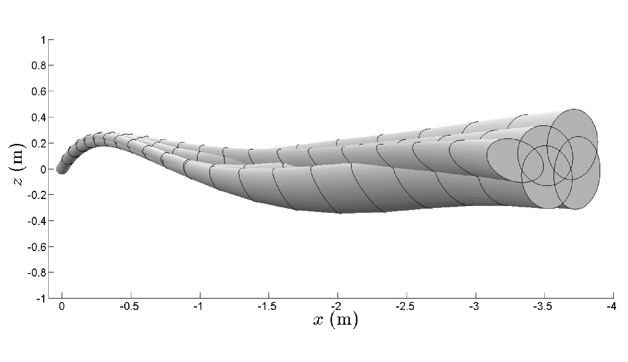
The funnel is both a certificate and a diagnostic. When it shrinks, the maneuver is fragile. When it grows, the controller has room to correct errors. In this glider, the shrinking is not a numerical artifact; it is the physics of low-speed, post-stall flight showing up in the certificate.
Lyapunov analysis with sums of squares: an alternative approach
Different from the equality-constrained formulation and rescaling strategy in Underactuated Robotics and its Van der Pol SOS pset, a more direct alternative is to use the standard SOS $S$-procedure over a sublevel set with an explicit decay margin. Start from a feasible quadratic seed, such as a Lyapunov equation or LQR design, then alternate two steps.
Step A — Multiplier certification. For fixed $V(\boldsymbol{x})$ and $\rho$, solve
\[\begin{aligned} \max_{\lambda(\boldsymbol{x}),\,s}\quad & s \\ \mathrm{s.t.}\quad & s>0,\\ & -\dot{V}(\boldsymbol{x}) + \lambda(\boldsymbol{x})\bigl(V(\boldsymbol{x})-\rho\bigr) - s \in \mathrm{SOS},\\ & \lambda(\boldsymbol{x})\in \mathrm{SOS}. \end{aligned}\]This certifies $\dot{V}(\boldsymbol{x})\le -s$ on the sublevel set $V(\boldsymbol{x})\le \rho$.
Step B — Lyapunov-function update. With the multiplier fixed, update $V$ while fixing its scale, for example by choosing a nonzero normalization point $\boldsymbol{x}_{\mathrm{scale}}$ and solving
\[\begin{aligned} \max_{V(\boldsymbol{x}),\,\rho}\quad & \rho \\ \mathrm{s.t.}\quad & \rho>0,\\ & V(\boldsymbol{0})=0, \qquad V(\boldsymbol{x}_{\mathrm{scale}})=1,\\ & V(\boldsymbol{x})-\epsilon\,\boldsymbol{x}^{\top}\boldsymbol{x} \in \mathrm{SOS},\\ & -\dot{V}(\boldsymbol{x}) + \lambda(\boldsymbol{x})\bigl(V(\boldsymbol{x})-\rho\bigr) \in \mathrm{SOS}. \end{aligned}\]The scale constraint is essential; otherwise searching over both $V$ and $\rho$ is underconstrained. Alternate the two steps until the certified region stabilizes. [code]
Model-Based Learning Perching
So far, the learning has been used to build a better model before planning. We identified a flat-plate baseline plus a compact residual model, then used that model for trajectory optimization, stabilization, and funnel analysis. A natural next step is to close that loop.
The glider should not only learn from old batches of flight data. It should use the model to plan a maneuver, fly the maneuver, notice how reality disagreed with the model, update the residual, and then plan again.
This is where iLQR fits naturally into the story.
Direct collocation asks for a feasible movie all at once. TVLQR stabilizes a fixed movie. iLQR sits between them: like TVLQR, it builds local linear-quadratic models along a nominal trajectory; unlike TVLQR, it uses those local models to update the nominal trajectory itself.
Around a current nominal trajectory $\boldsymbol{x}_0[\cdot],\boldsymbol{u}_0[\cdot]$, iLQR uses the same error-coordinate idea as TVLQR,
\[\bar{\boldsymbol{x}}[n] = \boldsymbol{x}[n]-\boldsymbol{x}_0[n], \qquad \bar{\boldsymbol{u}}[n] = \boldsymbol{u}[n]-\boldsymbol{u}_0[n].\]The local LQR step now has both a feedback term and a feedforward term:
\[\bar{\boldsymbol{u}}[n] = \boldsymbol{k}[n] - \boldsymbol{K}[n]\bar{\boldsymbol{x}}[n].\]The $-\boldsymbol{K}[n]\bar{\boldsymbol{x}}[n]$ term is the same local tracking correction as TVLQR, while $\boldsymbol{k}[n]$ is the feedforward step that moves the nominal trajectory. A forward rollout with this update produces a new nonlinear trajectory. Then the process repeats.
In the model-learning version of the perching problem, the planner uses
\[\dot{\boldsymbol{x}} = f_{\mathrm{fp}}(\boldsymbol{x},\boldsymbol{u}) + g(\boldsymbol{x},\boldsymbol{u})\boldsymbol{w}_j,\]where $f_{\mathrm{fp}}$ is the flat-plate model and $g(\boldsymbol{x},\boldsymbol{u})\boldsymbol{w}_j$ is the current aerodynamic residual. The residual may represent corrections to lift, drag, and pitching moment coefficients, but the important point is that it is still linear in the unknown weights.
At learning iteration $j$, the loop is
\[\begin{aligned} \text{Plan:}\qquad & \{\boldsymbol{x}^j[\cdot],\boldsymbol{u}^j[\cdot], \boldsymbol{k}^j[\cdot],\boldsymbol{K}^j[\cdot]\} = \mathrm{iLQR}\!\left(f_{\mathrm{fp}}+g\boldsymbol{w}_j\right),\\[1mm] \text{Execute:}\qquad & \boldsymbol{u}[n] = \boldsymbol{u}^j[n] + \boldsymbol{k}^j[n] - \boldsymbol{K}^j[n]\bigl(\boldsymbol{x}[n]-\boldsymbol{x}^j[n]\bigr),\\[1mm] \text{Identify:}\qquad & \boldsymbol{w}_{j+1} = \arg\min_{\boldsymbol{w}} \sum_{n=0}^{N-1} \left\| \dot{\boldsymbol{x}}_{\mathrm{data}}[n] - f_{\mathrm{fp}}(\boldsymbol{x}[n],\boldsymbol{u}[n]) - g(\boldsymbol{x}[n],\boldsymbol{u}[n])\boldsymbol{w} \right\|^2 + \gamma\|\boldsymbol{w}\|^2,\\[1mm] \text{Re-plan:}\qquad & \text{run iLQR again with } f_{\mathrm{fp}}+g\boldsymbol{w}_{j+1}. \end{aligned}\]The regression step is simple because the residual was designed to be linear in its weights. From the executed rollout,
\[\dot{\boldsymbol{x}}_{\mathrm{data}}[n] \approx \frac{\boldsymbol{x}[n+1]-\boldsymbol{x}[n]}{h},\]and the model error is fit as
\[\dot{\boldsymbol{x}}_{\mathrm{data}}[n] - f_{\mathrm{fp}}(\boldsymbol{x}[n],\boldsymbol{u}[n]) \approx g(\boldsymbol{x}[n],\boldsymbol{u}[n])\boldsymbol{w}.\]In practice, we fit only the components where the aerodynamics enter directly: the translational accelerations and the pitch acceleration. The rest of the state equations are mostly kinematic.


Extension: Zero-Order Methods for Perching
The previous sections followed the trajectory-optimization route: choose state and input samples explicitly, then enforce dynamics through collocation constraints. The same glider also gives a clean testbed for zero-order planners such as MPPI and CEM.
MPPI treats planning as repeated sampling, rollout, and soft selection. It keeps a nominal open-loop control sequence
\[\boldsymbol{U} = \{\boldsymbol{u}_0,\ldots,\boldsymbol{u}_{N-1}\},\]samples noisy variants of that sequence,
\[\boldsymbol{u}^{(j)}[n] = \boldsymbol{u}_0[n] + \boldsymbol{\epsilon}^{(j)}[n], \qquad \boldsymbol{\epsilon}^{(j)}[n] \sim \mathcal{N}(\boldsymbol{0},\boldsymbol{\Sigma}),\]rolls each candidate through the nonlinear glider model,
\[\boldsymbol{x}^{(j)}[n+1] = \boldsymbol{x}^{(j)}[n] + h\,f\!\left( \boldsymbol{x}^{(j)}[n], \boldsymbol{u}^{(j)}[n] \right),\]and scores the resulting trajectory,
\[J^{(j)} = \ell_f\!\left(\boldsymbol{x}^{(j)}[N]\right) + \sum_{n=0}^{N-1} h\,\ell\!\left( \boldsymbol{x}^{(j)}[n], \boldsymbol{u}^{(j)}[n] \right).\]In perching, this cost says: arrive near the perch with the right state. Some samples flare too early and fall short. Some stay fast too long and pass the target. A few discover the useful timing: carry enough speed, pitch up, generate drag, lose kinetic energy, and still keep enough authority to finish the maneuver.
The key difference from random shooting is that MPPI does not simply pick the best rollout. It forms a soft-min over sampled futures,
\[w^{(j)} = \frac{ \exp\!\left(-J^{(j)}/\lambda\right) }{ \sum_i \exp\!\left(-J^{(i)}/\lambda\right) },\]and updates the nominal control sequence by the weighted average of the sampled perturbations,
\[\boldsymbol{u}_0[n] \leftarrow \boldsymbol{u}_0[n] + \sum_j w^{(j)} \boldsymbol{\epsilon}^{(j)}[n].\]This is the computational heart of MPPI: low-cost rollouts pull the nominal control sequence toward themselves, while high-cost rollouts contribute almost nothing. The parameter $\lambda$ is the temperature. Small $\lambda$ makes the update colder and greedier, closer to choosing the best samples. Large $\lambda$ makes the update warmer and more conservative. The covariance $\boldsymbol{\Sigma}$ controls exploration in control-sequence space.
There is also a clean information-theoretic view. Let $p(\tau)$ be the baseline trajectory distribution induced by noisy control sequences and the dynamics, and let $q(\tau)$ be a new trajectory distribution. MPPI can be motivated by the tradeoff
\[\min_q \quad \mathbb{E}_q[J(\tau)] + \lambda\,\mathrm{KL}\!\left(q(\tau)\|p(\tau)\right),\]whose solution has the Gibbs / Boltzmann form
\[q^\star(\tau) \propto p(\tau) \exp\!\left(-J(\tau)/\lambda\right).\]The exact $q^\star$ is generally not Gaussian, because nonlinear dynamics and exponential cost weighting distort the sampled distribution. MPPI keeps a simple Gaussian family over control sequences and updates only its mean. In that sense, the weighted perturbation update is a practical moment-matching approximation to the low-cost trajectory distribution. [6]
For the glider, the appeal is practical: MPPI does not need derivatives of the post-stall aerodynamic model, does not solve a nonlinear program, and does not impose collocation constraints. It only needs fast rollouts and a task cost. That makes it a useful contrast to direct collocation: direct collocation searches through constrained decision variables; MPPI searches through sampled control histories.
The caveat is equally important. The Gaussian perturbations $\boldsymbol{\epsilon}^{(j)}[n]$ are search noise, not automatically physical uncertainty. They are not, by themselves, a model of wind, vortex shedding, or aerodynamic mismatch. Physical robustness comes either from running MPPI in a receding-horizon loop from the measured state, or from explicitly sampling uncertain dynamics during rollouts: different aerodynamic parameters, gusts, drag coefficients, or residual force models.
This perspective also connects to recent sampling-based MPC work such as DIAL-MPC, which views MPPI-like updates through a diffusion-style lens: broad sampling improves coverage, while smaller sampling noise improves local convergence. For perching, the same tradeoff appears naturally. Too little exploration never discovers the aggressive flare; too much exploration makes the update noisy. The planner has to balance coverage of possible futures with convergence to a precise landing maneuver. [7]

From the sampled rollout video, we can feel that the soft-min makes the update less brittle than picking a single best rollout: many good trajectories contribute, and poor trajectories are exponentially downweighted. But this is not, by itself, physical robustness to wind or model error. Physical robustness only appears if those uncertainties are included in the rollout distribution, or if the update is run in a receding-horizon loop from the measured state.
A short coda: path integrals and variational thinking
This formulation—finding the optimal trajectory by evaluating a distribution of all possible paths weighted by $\exp(-S/\lambda)$—is profound because it echoes a much deeper variational idea. If we replace our control cost with physical action and the temperature $\lambda$ with Planck’s constant, we step into Feynman’s path integral formulation, where the classical principle of least action emerges from a cloud of possible histories.
A beam of light enters water and bends. It almost looks as if the photon has foresight: I am about to enter water, where I will move more slowly, so I should spend a little more distance in air and a little less distance in water. The path looks planned, but there is no planner inside the photon.
Feynman gives the deeper picture. In the quantum picture, there is not only one path. From point $a$ to point $b$, the particle explores all possible paths. One can imagine the whole space filled with infinitely many Thomas Young double-slit experiments: every point is another possible slit, and every nearby route contributes a tiny arrow of probability amplitude.
The formal object is the path integral,
\[K(b,a) = \int \mathcal{D}\boldsymbol{q}(t)\, \exp\!\left(\frac{i}{\hbar}S[q]\right),\]where
\[S[\boldsymbol{q}] = \int L(\boldsymbol{q},\dot{\boldsymbol{q}},t)\,dt, \qquad L = T - V.\]The appearance of $T-V$ is not arbitrary. Energy is
\[H = T + V,\]but action is built from
\[\boldsymbol{p}^{\top}\dot{\boldsymbol{q}} - H.\]For ordinary mechanical systems, $\boldsymbol{p}^{\top}\dot{\boldsymbol{q}} = 2T$, so
\[\boldsymbol{p}^{\top}\dot{\boldsymbol{q}} - H = 2T-(T+V) = T-V.\]Now comes the beautiful cancellation picture. Each possible path carries a little complex arrow,
\[\exp(iS/\hbar).\]For most paths, if we perturb the path even slightly, the action changes quickly:
\[\delta S \neq 0.\]So nearby arrows point in wildly different directions,
\[\nearrow,\quad \leftarrow,\quad \searrow,\quad \uparrow,\quad \cdots\]and they cancel each other out.
But near special paths,
\[\delta S = 0.\]A small change in the path does not change the action to first order. The nearby arrows remain almost aligned, so they reinforce instead of cancel.
That surviving path is what we see as the classical path. Not because the photon knew the answer in advance, but because all the other paths destructively interfered away. Nature does not first choose one trajectory and then execute it. It lets all possible histories speak, and only the phase-consistent ones remain.
What is especially beautiful for robotics is that the same object reappears in multibody dynamics. When we derive robot dynamics, we also build
\[L(\boldsymbol{q},\dot{\boldsymbol{q}}) = T(\boldsymbol{q},\dot{\boldsymbol{q}}) - V(\boldsymbol{q}),\]and put it into the Lagrange equations. So the bending of light, the motion of particles, and the mechanics of robots are not separate miracles. They are different faces of the same variational structure: motion as a statement about paths.
References
[1] Russ Tedrake. Underactuated Robotics Ch.10 Trajectory Optimization Course Notes for MIT 6.832, 2023. [link]
[2] Russ Tedrake. Underactuated Robotics Ch.9 Lyapunov Analysis Sec.9.2 Lyapunov analysis with convex optimization Course Notes for MIT 6.832, 2023. [link]
[3] Russ Tedrake. Underactuated Robotics Ch.11 Policy Search Course Notes for MIT 6.832, 2023. [link]
[4] Joseph Moore. Learning based control for robotics Course Notes for JHU ME696, 2025. [link]
[5] Joseph Moore, “Robust Post-Stall Perching with a Fixed-Wing UAV”, PhD thesis, Massachusetts Institute of Technology, September, 2014. [link]
[6] Heng Yang. Optimal Control and Reinforcement Learning, Ch.4 Model-based Planning and Optimization. Textbook for Harvard ES/AM 158: Introduction to Optimal Control and Reinforcement Learning, 2025. [link]
[7]. Xue, H., Pan, C., Yi, Z., Qu, G., and Shi, G. Full-Order Sampling-Based MPC for Torque-Level Locomotion Control via Diffusion-Style Annealing. In 2025 IEEE International Conference on Robotics and Automation (ICRA), pp. 4974–4981, 2025. [link]