Continuous-time Successive Convexification
TL;DR
Conventional direct transcription methods enforce path constraints only at a finite set of nodes. A trajectory can therefore look feasible on the optimization grid while violating safety constraints between samples. This project reproduces the main idea of Continuous-Time Successive Convexification (CT-SCVX): convert continuous-time path-constraint violation into an augmented state, linearize the resulting exact flow map with variational ODEs, and solve a sequence of convex subproblems. I first reproduce the continuous-time constraint-satisfaction idea on obstacle avoidance, then extend it to a constrained cart-pole swing-up problem. The key lesson is not merely denser discretization, but a different object of optimization: the solver sees an accumulated continuous-time violation, and every candidate trajectory is checked by nonlinear rollout.
Nonlinear optimal control is naturally a continuous-time problem. We want a trajectory satisfying
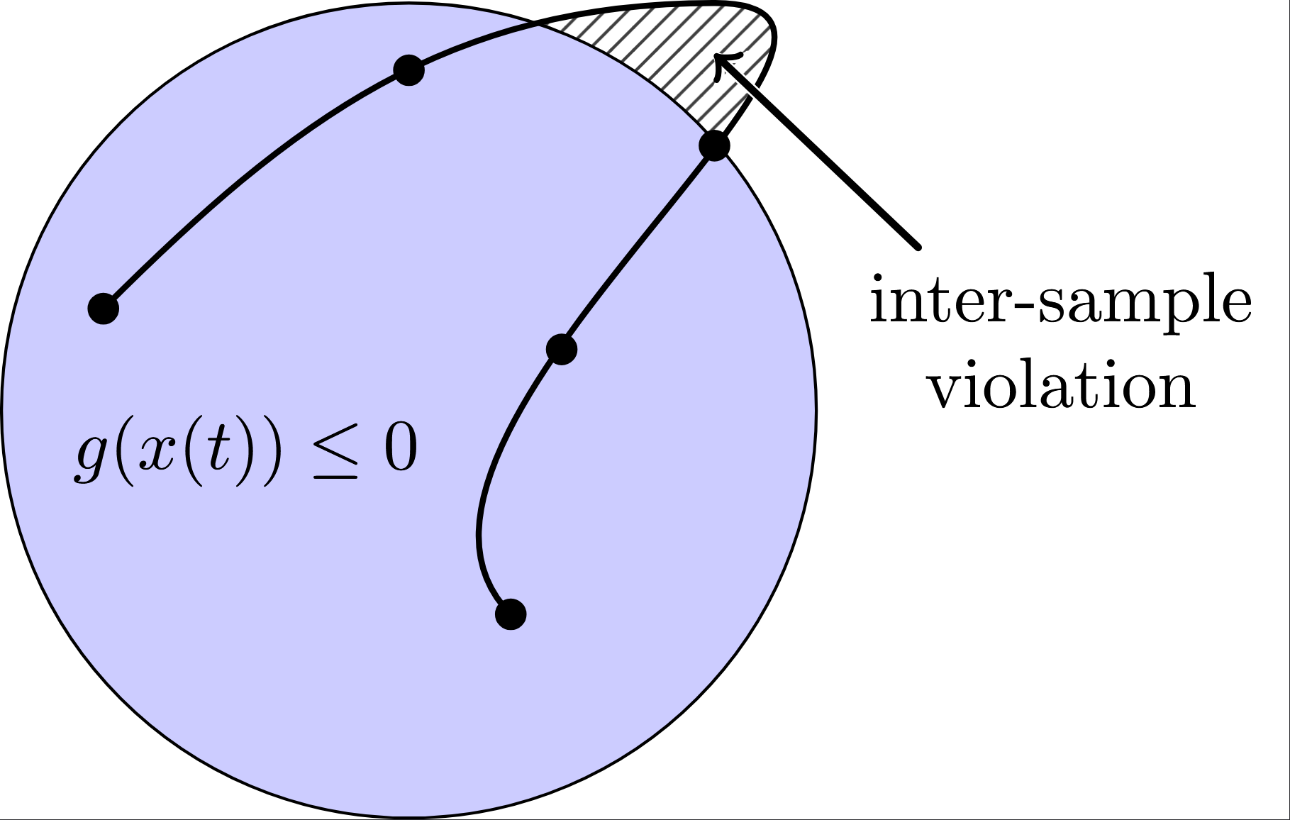
\[\dot{x}(t)=f(x(t),u(t)), \qquad g(x(t),u(t))\le 0, \qquad t\in[0,t_f].\]Direct methods make this finite-dimensional by choosing a grid and optimizing over the nodal states and controls. This is computationally attractive, but it creates a subtle failure mode: enforcing $g(x_k,u_k)\le 0$ only at the nodes says almost nothing about what happens inside each interval. In obstacle avoidance, rocket landing, or constrained swing-up, that gap can be the difference between a valid trajectory and one that is only discretely feasible.
Problem Formulation
Consider a fixed-final-time nonlinear optimal control problem in Mayer-Bolza form:
\[\begin{aligned} \min_{x(\cdot),u(\cdot)} \quad & \int_0^{t_f} L(x(t),u(t))\,dt + L_f(x(t_f)) \\ \text{s.t.}\quad & \dot{x}(t)=f(x(t),u(t)), && t\in[0,t_f],\\ & g(x(t),u(t))\le 0, && t\in[0,t_f],\\ & u(t)\in\mathcal U, && t\in[0,t_f],\\ & x(0)=x_0, \qquad \psi(x(t_f))=0. \end{aligned}\]Here $x(t)\in\mathbb R^{n_x}$ is the state, $u(t)\in\mathbb R^{n_u}$ is the control, $f$ is the nonlinear vector field, $g$ is the vector of path constraints, and $\mathcal U$ is a simple convex control set. In the original CT-SCVX paper, free-final-time problems can be handled by time-dilation. For this cart-pole project, I use a fixed final time, so the essential idea can be written without introducing the dilation factor.
Define the squared-hinge exterior penalty
\[\Lambda(x,u)=\frac12\|[g(x,u)]_+\|_2^2,\qquad [g]_+:=\max\{g,0\}\text{ componentwise}.\]This penalty is nonnegative, and $\Lambda(x,u)=0$ if and only if all inequality path constraints are satisfied at that state-control pair. Introduce an accumulated violation state and a running-cost state,
\[y(t)=\int_0^t \Lambda(x(\tau),u(\tau))\,d\tau,\qquad w(t)=\int_0^t L(x(\tau),u(\tau))\,d\tau,\]and define the augmented state
\[\bar{x}=\begin{bmatrix}x\\y\\w\end{bmatrix},\qquad \dot{\bar{x}}=\bar f(\bar{x},u)= \begin{bmatrix} f(x,u)\\ \Lambda(x,u)\\ L(x,u) \end{bmatrix},\qquad \bar{x}(0)=\begin{bmatrix}x_0\\0\\0\end{bmatrix}.\]The reason this is powerful is simple. Since $\Lambda\ge 0$, exact continuous-time feasibility is equivalent to
\[y(t_f)=\int_0^{t_f}\Lambda(x(t),u(t))\,dt=0.\]If the integral of a continuous nonnegative violation function is zero, then the violation must be zero everywhere except possibly on a measure-zero set; under the usual continuity of $g(x(t),u(t))$, this rules out hidden inter-sample constraint violation. In computation, we use a small tolerance, for example $y(t_f)\le\delta_y$, and then verify the trajectory with a high-accuracy nonlinear rollout and dense samples of $g(x(t),u(t))$.
Multiple-Shooting Discretization & First-Order Sensitivities via Variational ODEs
Choose a fixed time grid $0=t_1<t_2<\cdots<t_N=t_f$ and use zero-order-hold controls
\[u(t)=\eta_k, t\in[t_k,t_{k+1}), k=1,\ldots,N-1.\]Let $\xi_k\in\mathbb R^{n_{\bar x}}$ denote the augmented shooting state at node $t_k$. For each interval, define the exact augmented flow map
\[F_k(\xi_k,\eta_k)=\bar{x}(t_{k+1}),\]where $\bar{x}(t)$ solves IVP $\dot{\bar{x}}(t)=\bar f(\bar{x}(t),\eta_k), \bar{x}(t_k)=\xi_k.$
The nonlinear multiple-shooting constraints are then $\xi_{k+1}=F_k(\xi_k,\eta_k),\quad k=1,\ldots,N-1.$
The advantage of this transcription is that the dynamics inside each interval are still represented by the continuous-time flow map. The grid gives us decision variables, but the interval transition itself comes from integrating the ODE, up to the numerical tolerance of the ODE solver.
At each SCP iteration, the flow map is linearized around the current nominal trajectory $(\tilde\xi_k,\tilde\eta_k)$. Since $F_k$ is defined by an ODE solve, finite-differencing it would be slow and often inaccurate. CT-SCVX instead integrates the augmented dynamics and their variational equations in one enlarged ODE:
\[\begin{aligned} \dot{\bar{x}}(t) &= \bar f(\bar{x}(t),\tilde\eta_k), & \bar{x}(t_k)&=\tilde\xi_k,\\ \dot\Phi_{\bar{x}}(t) &= \bar f_{\bar{x}}(\bar{x}(t),\tilde\eta_k)\Phi_{\bar{x}}(t), & \Phi_{\bar{x}}(t_k)&=I,\\ \dot\Phi_u(t) &= \bar f_{\bar{x}}(\bar{x}(t),\tilde\eta_k)\Phi_u(t)+\bar f_u(\bar{x}(t),\tilde\eta_k), & \Phi_u(t_k)&=0. \end{aligned}\]The terminal values give the first-order sensitivity matrices $A_k=\Phi_{\bar{x}}(t_{k+1}),\qquad B_k=\Phi_u(t_{k+1}),$ with $\tilde F_k=F_k(\tilde\xi_k,\tilde\eta_k),\quad d_k=\tilde F_k-A_k\tilde\xi_k-B_k\tilde\eta_k,$ the local affine model ism$F_k(\xi_k,\eta_k)\approx A_k\xi_k+B_k\eta_k+d_k.$
Therefore the affine shooting residual used in the convex subproblem is $\hat r_k(Z)=\xi_{k+1}-A_k\xi_k-B_k\eta_k-d_k.$
This is the computational core of the method: the nonlinear dynamics and continuous-time violation state are integrated once per interval around the nominal trajectory; the optimizer then sees a fixed affine flow model.
One subtle issue in the original CT-SCVX formulation is the boundary condition on the violation accumulator. If one directly enforces both the augmented dynamics and $y_{k+1}-y_k=0$, then at exact feasibility the derivative of the squared-hinge violation can vanish, causing a redundant active constraint and a LICQ failure. The original method therefore relaxes this condition to
\[y_{k+1}-y_k\le \epsilon,\qquad \epsilon>0,\]or equivalently uses a small violation budget. This is not a philosophical weakening of the method; it is a numerical and variational device that keeps the reformulated problem well-posed. In the limit of small $\epsilon$, the continuous-time violation is driven to zero, and in practice the final trajectory is judged by true rollout, terminal error, accumulated $y(t_f)$, and dense constraint samples.
The relaxed multiple-shooting problem can be summarized as
\[\begin{aligned} \min_{\xi_{1:N},\eta_{1:N-1}} \quad & w_N+L_f(E_x\xi_N) \\ \text{s.t.}\quad & \xi_{k+1}=F_k(\xi_k,\eta_k), && k=1,\ldots,N-1,\\ & y_{k+1}-y_k\le\epsilon, && k=1,\ldots,N-1,\\ & \eta_k\in\mathcal U, && k=1,\ldots,N-1,\\ & \xi_1=\begin{bmatrix}x_0\\0\\0\end{bmatrix},\\ & E_x\xi_N=x_f. \end{aligned}\]Here $E_x$ extracts the physical state from the augmented state. For the cart-pole implementation, I found it more robust to begin with a strong soft terminal penalty and switch to a hard terminal equality only during a polishing phase.
$\ell_1$ Exact Penalization and the Prox-Linear Method
After multiple shooting, the continuous-time OCP becomes a finite-dimensional nonlinear program. The original CT-SCVX method solves it with a prox-linear algorithm applied to an exact-penalty reformulation. The nonlinear shooting equality is first moved into the objective through an $\ell_1$ exact penalty, $J(z)+\gamma\sum_{k=1}^{N-1}|\xi_{k+1}-F_k(\xi_k,\eta_k)|_1$, where $z$ stacks all shooting states and controls.
At SCP iteration $i$, the nonlinear flow map is replaced by its affine approximation,
\[\hat r_k^i(z) = \xi_{k+1}-A_k^i\xi_k-B_k^i\eta_k-d_k^i,\]and the local prox-linear model becomes
\[J_i(z)+\gamma\sum_{k=1}^{N-1}\|\hat r_k^i(z)\|_1 +\frac{1}{2\rho}\|z-\tilde z^i\|_2^2.\]The $\ell_1$ term is implemented with nonnegative positive and negative slack variables: $\hat r_k^i(z)=q_k-r_k$, $q_k\ge 0$, $r_k\ge 0$, and $|\hat r_k^i(z)|_1=\mathbf 1^\top(q_k+r_k)$. Thus each CT-SCVX step solves a convex subproblem of the form
\[\begin{aligned} \min_{\xi,\eta,q,r}\quad & J_i(\xi,\eta) +\gamma\sum_{k=1}^{N-1}\mathbf 1^\top(q_k+r_k) +\frac{1}{2\rho}\|z-\tilde z^i\|_2^2\\ \text{s.t.}\quad & \hat r_k^i(z)=q_k-r_k,\qquad k=1,\ldots,N-1,\\ & q_k\ge 0,\quad r_k\ge 0,\\ & y_{k+1}-y_k\le \epsilon,\\ & \eta_k\in\mathcal U,\qquad \xi_1=\begin{bmatrix}x_0\\0\\0\end{bmatrix}. \end{aligned}\]The proximal term keeps the new iterate close to the trajectory around which the flow map was linearized. It’s therefore both a regularizer and a trust-region mechanism.
Also, compared with a static $\gamma\ell_1$ exact penalty, ALM is a primal-dual method, it carries multipliers for the residual constraints and updates them from the observed constraint violation. This avoids relying on a manually chosen large penalty weight to force feasibility. For affine shooting residuals $\hat r_k^i(z)$, the ALM subproblem replaces the $\ell_1$ term by
\[\sum_{k=1}^{N-1} \left[ (\lambda_k^i)^\top \hat r_k^i(z) + \frac{\mu_i}{2}\|\hat r_k^i(z)\|_{W_r}^2 \right],\]leading to a convex QP of the form
\[\begin{aligned} \min_{\xi,\eta}\quad & J_i(\xi,\eta) +\sum_{k=1}^{N-1} \left[ (\lambda_k^i)^\top \hat r_k^i(z) + \frac{\mu_i}{2}\|\hat r_k^i(z)\|_{W_r}^2 \right] +\frac{1}{2\rho}\|z-\tilde z^i\|_2^2\\ \text{s.t.}\quad & 0\le y_k\le \delta_y,\qquad k=1,\ldots,N,\\ & \eta_k\in\mathcal U,\qquad \xi_1=\begin{bmatrix}x_0\\0\\0\end{bmatrix}. \end{aligned}\]After the QP is solved, the candidate is checked against the true nonlinear dynamics, not only the affine model. The controls are rolled out through the original continuous-time system, and the terminal error, accumulated violation, dense path-constraint margins, and true shooting residuals are evaluated. Only after a candidate is accepted are the multipliers updated as $\lambda_k^{i+1}=\lambda_k^i+\mu_i W_r r_{k,\mathrm{true}}^{i,+}$.
To validate this framework above, project evaluate it on two optimal control tasks. The first is a 2D double-integrator obstacle-avoidance problem. The node-only baseline (classic direct transcription formulation) satisfies the obstacle constraint at the grid points only, but its continuous trajectory by higher accuracy simulator can pass through the obstacle between nodes. In contrast, the optimized trajectory of CT-SCVX formulation above stays outside the exclusion region under dense rollout evaluation. Figure on the right shows the constraint violation in continuous time under higher accuracy simulator (high-order differential equation integrator). [ code →]


The second example is the cart-pole swing-up with tight cart and pole-tip box constraints. This is a useful small extension because the system is nonlinear, underactuated, and easy to solve incorrectly: a node-only transcription can satisfy the constraints at the samples while the pole tip leaves the permitted box between sample nodes. In the CT-SCVX/ALM version, the path constraints are encoded through the accumulated violation state $y$, and the final trajectory is judged only after high-accuracy nonlinear rollout. The resulting swing-up is more conservative than a purely node-constrained solution, but its continuous-time constraint margins are substantially more reliable. The figure below shows the pole-tip box-constraint violation under dense evaluation.
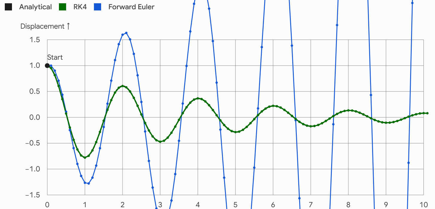
During the swing-up, the dynamics can amplify accumulated integration and transcription errors. This is especially true when the pole moves from angle $\pi/2$ toward $\pi$ (especially $\pi/2$ in [3] and interestingly cartpole exactly fails at $\pi/2$ for node-only control policy in simulation in following trajectory figure, light blue curve), where the cart has poor instantaneous authority over the pole (see [3], Prof. Tedrake have detailed explanation on why trajectory stabilization matters). In this region, even a small mismatch between the simulated state and the nominal trajectory can be amplified significantly, causing the open-loop rollout to miss the swing-up.
However, interestingly the CT-SCVX/ALM is seccessful in doing the swing-up with the open-loop control policy directly throw into the higher accuracy simulator with the same ZOH frequency. That’s because the continuous time dynamics is satisfied almost everywhere over the entire time horizon and can work even without trajectory stablization. And the violation of the holonomic constraints remains negligible.

Discussion on trajectory optimization
[3] has beautiful insights on trajectory optimization (intuition on trajopt v.s. DP and Lyapnov; comparision between shooting and different direct transcription method; trajectory stablization after trajectory finding). Additionally, Drake provides a variety of numerical integrators at different levels as discussed earlier. Some of the algorithms detailed in [3] are presented below: [ code →]
Direct Transcription
Backpropagation
DDP
iLQR
Possible and creative future work can be to make the time grid itself part of the trajectory optimization. Instead of fixing a uniform step size, we can optimize the interval lengths $h_k = t_{k+1}-t_k$ together with the states and controls. This allows the optimizer to spend more resolution where the dynamics are fast or highly nonlinear, and use larger steps where the motion is smooth. A particularly interesting version is to borrow the error-estimation idea from RK45. For each interval, we can compute both a RK fourth-order forward pass and a fifth-order update,
\[x_{k+1}^{(4)}=\Phi^{(4)}(x_k,u_k,h_k), \quad x_{k+1}^{(5)}=\Phi^{(5)}(x_k,u_k,h_k),\]and constrain their difference (on $x_k,u_k,h_k$),
\[\left\| \Phi^{(5)}(x_k,u_k,h_k) - \Phi^{(4)}(x_k,u_k,h_k) \right\| \leq \epsilon .\]The solver is no longer to hide variable-step logic inside the constraint, but it can explicitly choose smaller $h_k$ where the integration error would be large. In this way, the optimizer simultaneously designs the trajectory, allocates time, and controls numerical accuracy.
References
[1]. Yue Yu. Numerical Trajectory Optimization. Course notes for UMN AEM 5431.
[2]. Elango, P., Luo, D., Kamath, A. G., Uzun, S., Kim, T., & Açıkmeşe, B. Continuous-time successive convexification for constrained trajectory optimization. Automatica, vol. 180, Art. no. 112464, Oct. 2025. doi:10.1016/j.automatica.2025.112464. [link]
[3]. Russ Tedrake. Underactuated Robotics, Chapter 10: Trajectory Optimization. Course notes for MIT 6.832. [link]